In a bladder-cytology segmentation project, the task is to label each pixel as nucleus, cytoplasm, or background. Once the nucleus and cytoplasm are separated, one can estimate the nucleus-to-cytoplasm (N/C) ratio, a key morphologic criterion in urinary cytology for assessing high-grade urothelial carcinoma. Doing that well requires more than the raw RGB triple at each pixel: an isolated colour does not tell you whether you are looking at a nucleus boundary, textured chromatin inside a nucleus, or smooth cytoplasm. Those distinctions are properties of neighbourhoods, not of single pixels — which is exactly what a feature map captures: a new image, the same size as the input, where each value summarises the pattern present in a small patch around the corresponding input pixel.
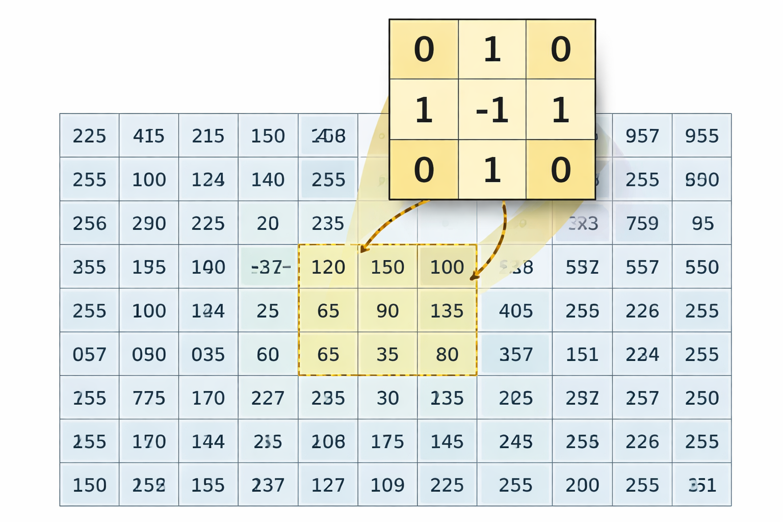
The filters below are also the right conceptual bridge to convolutional neural networks. Most of them take a small neighborhood — a kernel sliding across the image — and produce a feature map emphasizing a particular signal: smoothness, boundaries, or texture. The mechanic is the same for every linear filter in this chapter: centre the kernel on a pixel, multiply each kernel weight by the image value directly beneath it, sum those nine products, and write the single resulting number into the output feature map at that pixel. Slide the kernel one position over and repeat. The output ends up the same shape as the input, but each value now reports how strongly the pattern encoded by the kernel is present at that location. Different kernels emphasise different patterns; CNNs generalize this idea by learning the best kernels from data. Studying handcrafted filters first makes that leap concrete.
A 3×3 kernel hovering over an image, computing a dot product at each pixel position.
7.2 The Kernel Convolution Widget
Before exploring specific filters, build intuition for how any linear filter works. The widget shows a 3×3 kernel sliding over a small image of pixel values (0–1). Edit the kernel weights and watch the output feature map update live.
How to use: Click any pixel to see the dot-product breakdown. Edit the nine kernel weights to define any 3×3 filter. Use the preset buttons to load common filters — the active preset is highlighted blue. Click ▶ Play to animate the kernel scan row by row (the output feature map fills in live). Use Prev / Next to step manually, or ⏮ to reset.
The key insight: changing the kernel weights changes what the feature map emphasizes. CNNs learn these weights automatically from data.
7.3 Padding: What Happens at the Image Border
When you click the corner of the image in the widget above, the kernel’s 3×3 window cannot fit entirely inside the image — there are no pixels at row \(-1\) or column \(8\). To compute an output value at every input position, we have to invent values for the missing positions. The choice of how to invent them is called the padding mode.
Zero-padding — what the widget does. The faint grey halo of 0.00 cells around the 8×8 image is not decoration: it is the implicit border the widget uses whenever the kernel pokes off the image. Off-image positions contribute \(w \times 0 = 0\) to the dot product, and the readout panel marks those terms with a small pad subscript so you can see exactly which contributions came from the border. With a 3×3 kernel and a single ring of zero-padding, the output stays the same shape as the input (8×8). This is called “same” convolution.
Output size formula. For a 1-D image of length \(n\), kernel size \(k\), padding \(p\) (added to each side), and stride 1, the output length is \[\text{out} = n - k + 2p + 1.\]
Plug in \(n=8, k=3, p=1\) and you get \(\text{out}=8\) (the same convolution the widget does). Drop padding entirely (\(p=0\)) and the output shrinks: \(\text{out}=6\).
Three common alternatives.
Valid (no padding). Only positions where the kernel fully fits inside the image are computed; the output shrinks (\(8\times 8 \to 6\times 6\) for a 3×3 kernel). The manual-convolution snippet you’ll see in chapter 8 uses this mode.
Reflect. Mirror the image across the border, so pixel(-1, c) becomes pixel(1, c). This avoids the artificial darkening that zero-padding imposes on a blur kernel near edges, because the reflected pixel has roughly the same intensity as its neighbour.
Replicate (edge). Copy the boundary pixel outward, so pixel(-1, c) becomes pixel(0, c). Cheaper than reflect and very common in image-processing libraries.
In PyTorch, the option nn.Conv2d(..., padding=1) is exactly the zero-padding mode you saw here; that is why every convolution in chapter 8’s MinimalCNN keeps its feature maps at \(256 \times 256\).
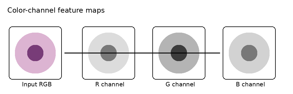
7.4 Raw Intensity and Color-Channel Maps
Color-channel feature maps
Before you engineer any feature, notice that the image already hands you a few for free. Every pixel comes with one or more numbers attached to it, and each of those numbers is itself a feature map — a value defined at every \((x,y)\) location.
These are your base channels, the raw input to everything that follows in this chapter. If a grayscale image is enough to separate nucleus from cytoplasm from background, you may not need to engineer anything else. More often, you’ll use them as the starting material that the filters below transform into something more discriminative.
What you get for free:
Grayscale image: a single intensity map \(I(x,y)\).
Color image: three maps stacked together, \[I(x,y) = \big(R(x,y),\,G(x,y),\,B(x,y)\big)\] Each channel — red, green, blue — is its own feature map you can feed to a classifier.
What you can derive without filtering. A few simple recombinations of the channels are still “free” features in the sense that no neighborhood operation is involved — you’re just remixing the numbers at each pixel:
A grayscale projection, \[Y(x,y)=0.2126\,R(x,y)+0.7152\,G(x,y)+0.0722\,B(x,y),\] which collapses color into a single brightness map.
A conversion from RGB to HSV, giving you hue \(H(x,y)\), saturation \(S(x,y)\), and value \(V(x,y)\) as three new candidate maps. Stained nuclei often pop out in saturation even when they look similar to cytoplasm in brightness.
Why this is the right place to start. For your nucleus / cytoplasm / background problem:
Nucleus often differs from cytoplasm by darkness or stain concentration — visible in \(I\) or \(V\).
Cytoplasm may separate more cleanly in one color channel than another.
Background is often relatively uniform in value or saturation.
So before reaching for a Sobel edge map or a Gabor filter, ask yourself: which channel already gives the cleanest visual separation between the three classes? That channel becomes your baseline feature, and every engineered feature from here on is judged by whether it adds something the raw channels missed.
Quiz: Raw Channels as Features
When we say a grayscale image’s intensity \(I(x,y)\) is itself a feature map, what does that imply about the role of raw channels in feature engineering?
Quiz: HSV Saturation
A staining protocol leaves nuclei a deep purple while the cytoplasm is pale pink and the background is white. Why might converting to HSV and using the saturation map \(S(x,y)\) help separate these regions, even when the brightness alone does not?
7.5 Gaussian Blur and Mean Blur
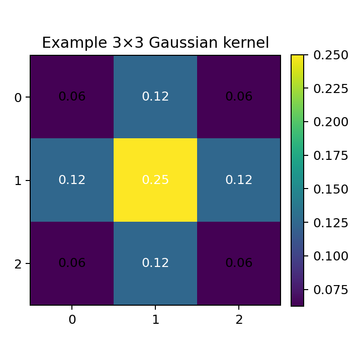
Example 3×3 Gaussian kernel
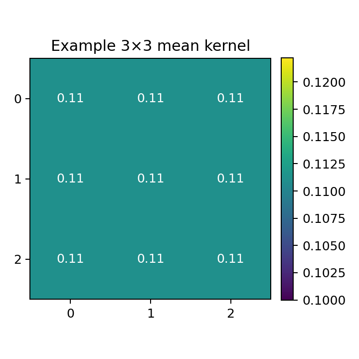
Example 3×3 mean kernel
These are the clearest examples of a kernel sliding across the image — exactly what the widget above demonstrates.
A mean blur with kernel \(K\) computes: \[F(x,y)=(K * I)(x,y)=\sum_{u=-r}^{r}\sum_{v=-r}^{r} K(u,v)\,I(x-u,y-v)\]
For a \(3\times 3\) mean filter: \[K_{\text{mean}}=\frac{1}{9}
\begin{bmatrix}
1&1&1\\
1&1&1\\
1&1&1
\end{bmatrix}\]
A Gaussian blur uses a kernel whose values follow a 2D normal distribution: \[G_\sigma(u,v)=\frac{1}{2\pi\sigma^2}\exp\!\left(-\frac{u^2+v^2}{2\sigma^2}\right)\]
Why this matters:
Reduces random pixel noise before stronger feature extraction.
Produces a coarse low-frequency map that separates broad cell regions from background.
Makes downstream edge maps more stable.
Caution
Too much blur weakens the boundaries you want to preserve. Apply conservatively, and always before edge detection.
The chapter recommends applying a Gaussian blur before computing edge or texture features. What is the primary reason?
Quiz: Gaussian vs Mean Kernel
Both the mean and Gaussian filters compute a weighted sum of pixels in a sliding window. What is the essential difference between their kernels?
7.6 Median and Rank Filters
Unlike mean and Gaussian blur, a median filter does not multiply and sum — it sorts the values in a local window and picks the middle one. This single difference makes it remarkably effective at removing isolated noise spikes without blurring edges.
7.6.1 How it works — step by step
For every output pixel, the filter:
Places a 3×3 window centred on that pixel — collecting 9 values.
Example — a salt spike (value 9) buried in the nucleus (value 1):
Step
Values
Window contents
1, 1, 1, 1, 9, 1, 1, 1, 1
Sorted
1, 1, 1, 1, 1, 1, 1, 1, 9
Output (rank 5)
1 ✓ spike removed
A mean filter would give \(\frac{8\times1+9}{9} \approx 1.9\) — a residual artifact. The median gives exactly 1, because the spike is pushed to the end of the sorted list and never reaches rank 5.
Example — a pepper spike (value 0) in the bright background (value 8):
Step
Values
Window contents
8, 8, 8, 8, 0, 8, 8, 8, 8
Sorted
0, 8, 8, 8, 8, 8, 8, 8, 8
Output (rank 5)
8 ✓ spike removed
7.6.2 Interactive Median/Rank Filter Explorer
The grid below uses values 0–9 (0 = black, 9 = white), matching the real staining convention: nucleus = 1 (dark), cytoplasm = 5 (medium), background = 8 (bright). Two noise spikes are planted: a salt spike at row 3, col 4 (value 9 in the dark nucleus — click it first) and a pepper spike at row 7, col 3 (value 0 in the bright background). Click any pixel to see its 3×3 window, the sorted values, and the median output. Click ▶ Play to animate the filter scan pixel by pixel (output fills in live), or use Prev / Next to step manually.
7.6.3 Rank filters — a generalisation
A rank filter returns the k-th ordered value rather than always the median:
Excellent at suppressing impulse noise (salt-and-pepper artifacts).
More edge-preserving than mean blur — the output is always one of the actual neighborhood values, never a blend.
Cleans isolated specks in the background while keeping cell boundaries sharp.
Note
Unlike mean and Gaussian blur, the median filter cannot be written as a convolution \(K * I\) with a fixed kernel — it is inherently nonlinear. This is why it does not appear as a preset in the kernel widget above.
Load Sobel X or Sobel Y in the widget to see how these kernels respond to edges in the example image.
Why this matters:
Highlights nucleus boundaries and cell boundaries directly.
Bright responses in \(M\) align with visible contours in the image.
One of the most interpretable handcrafted maps for segmentation.
Caution
Derivative-based maps are noise-sensitive. Apply a Gaussian blur first.
7.7.1 Live Sobel on a Real Cell Image
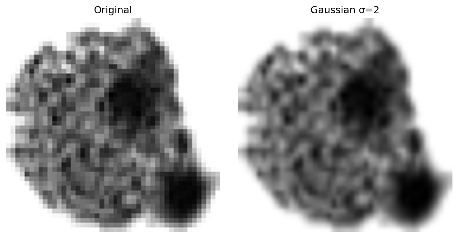
Pick a cell from the dropdown, then slide between \(G_x\), \(G_y\), and the gradient magnitude \(|G|\). Increase the pre-blur σ to see how Gaussian smoothing tames noise before differentiation. Every combination has been pre-rendered at build time so the slider feels live.
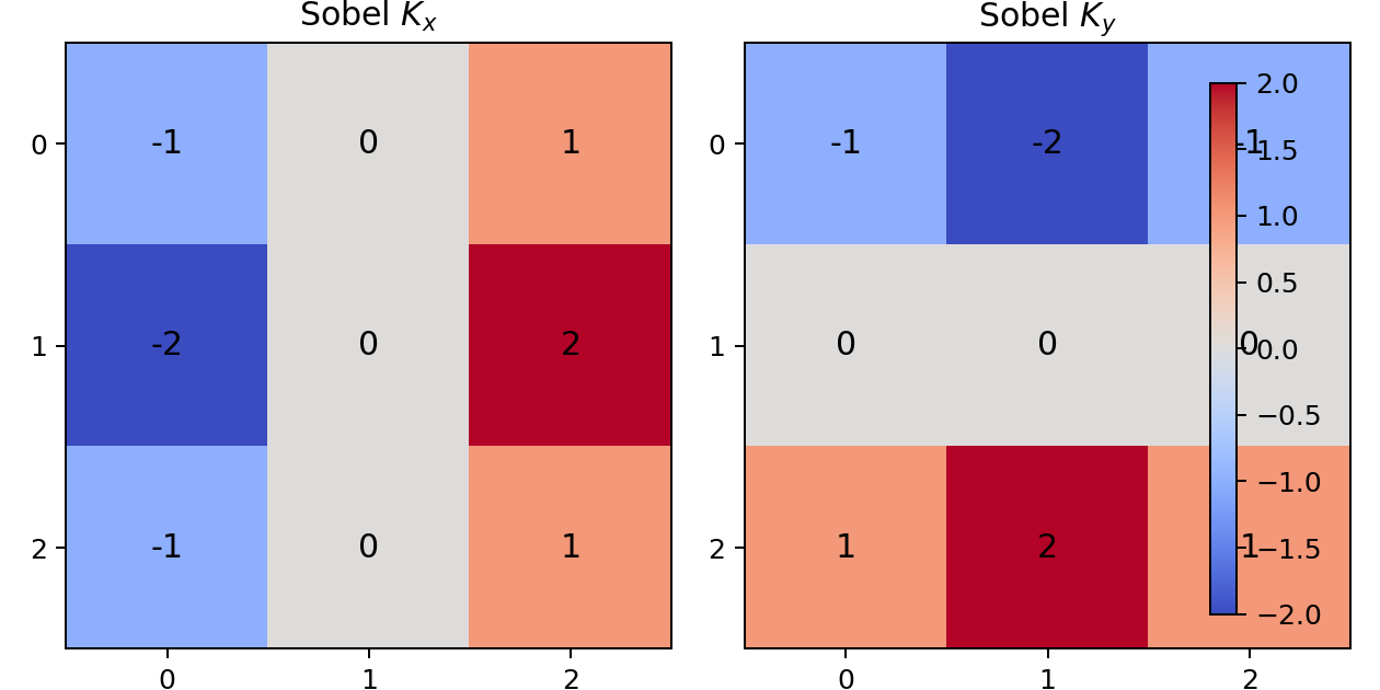
The Sobel operator computes \(G_x\) and \(G_y\) with two separate kernels, then combines them into a magnitude map \(G = \sqrt{G_x^2 + G_y^2}\). What does a high value in this magnitude map indicate?
Quiz: Sobel Noise Sensitivity
The chapter cautions that Sobel is “noise-sensitive” and recommends applying a Gaussian blur first. Why are derivative filters like Sobel especially vulnerable to noise?
7.8 Gabor Filters
A Gabor filter is a Gaussian-modulated sinusoid — it detects texture at a specific orientation and spatial frequency. Where Sobel detects any edge regardless of frequency, Gabor responds selectively to periodic patterns (e.g., chromatin texture in a nucleus).
7.8.1 From Formula to Matrix: Sampling a Continuous Function
A common point of confusion: the Gabor formula looks abstract, but it is just a recipe for filling in a kernel matrix. The same principle applies to the Gaussian kernel — both are continuous functions that you evaluate at discrete integer pixel offsets to produce the actual numbers in the sliding window.
For a 3×3 kernel, the offsets are \((a, b) \in \{-1, 0, +1\} \times \{-1, 0, +1\}\), where \(a\) is the row offset (negative = up, positive = down) and \(b\) is the column offset (negative = left, positive = right). Plug each pair into the formula to get the corresponding matrix entry:
The Gaussian envelope (\(\exp\) term) weights entries by distance from center — full weight at \((0,0)\), tapering toward the edges. This is exactly like a Gaussian blur kernel.
The sinusoidal wave (\(\cos\) term) creates alternating positive and negative bands across the kernel. \(\lambda\) sets the band width; \(\theta\) controls which direction the bands run.
Multiply the two and you get a kernel that responds to a specific texture frequency at a specific orientation.
7.8.2 What θ Does: Rotating the Stripe Pattern
The angle \(\theta\) rotates the coordinate system before the cosine is applied. At θ = 0°, \(x' = a\) (the row direction), so the cosine varies across rows → horizontal bands. At θ = 90°, \(x' = b\) (the column direction), so the cosine varies across columns → vertical bands.
Here are the two kernels computed from the formula with \(\lambda=2\), \(\sigma=1\), \(\gamma=1\):
\(K_{0°}\) fires when the center row is bright and the rows above and below are dark — a horizontal band crossing the kernel. \(K_{90°}\) fires when the center column is bright and the columns left and right are dark — a vertical band. Notice they are transposes of each other; rotating by 90° is equivalent to transposing the matrix.
For diagonal orientations (45°, 135°), the stripe pattern tilts, but a 3×3 grid is too coarse to display the diagonal clearly. A 5×5 kernel makes the orientation far more legible — which is why the widget below uses 5×5.
7.8.3 The Other Three Parameters
Parameter
Concrete meaning
Smaller value
Larger value
\(\lambda\)
Stripe width (wavelength)
Tight stripes — detects fine texture
Wide stripes — detects coarse texture
\(\sigma\)
Gaussian bell width
Small window, few stripes visible
Large window, more stripes captured
\(\gamma\)
Aspect ratio of the Gaussian ellipse
Elongated along the stripe direction
More circular envelope
A useful rule of thumb: keep \(\sigma \approx \lambda / \pi\) so that roughly one full stripe cycle fits within the Gaussian envelope.
7.8.4 Interactive Gabor Explorer
Edit the 10×10 image (click any cell to change its value), then drag the sliders to see the 5×5 kernel and its output feature map update live.
The default image has horizontal stripes — try θ = 0° first, then rotate to 90° and watch the output respond differently. Red cells in the output mean a strong positive match; blue cells mean a strong negative response (the inverse of the target texture).
How to use: Drag θ from 0° to 90° and watch the kernel’s stripe pattern rotate — the output’s bright-red regions shift accordingly. Try λ = 2 for tight stripes vs λ = 6 for wide ones. Increase σ to widen the Gaussian envelope and let more rows contribute. Click any input cell to type a new value (0.0–1.0), then draw your own texture and observe how the output responds.
Load the Gabor (0°) preset in the kernel convolution widget at the top of the chapter to see this same 3×3 version applied to the fixed example image.
7.8.5 Gabor Filter Banks
In practice a filter bank is used: multiple Gabor filters at several orientations (0°, 45°, 90°, 135°) and scales. Each filter produces one feature map. Together they form a rich multi-channel texture descriptor.
Why this matters for nucleus / cytoplasm / background:
Nucleus has distinctive chromatin texture — fine-grained periodic patterns visible at specific orientations and frequencies.
Cytoplasm is smoother and less structured.
Background is largely uniform, responding weakly to all Gabor filters.
A Gabor filter bank can distinguish these regions where Sobel or blur alone cannot.
Note
Gabor filters are linear convolutions — they are fixed kernels applied via \(F = K_{\text{Gabor}} * I\). A CNN trained on texture data tends to learn filters that closely resemble Gabor kernels in its early layers.
7.8.6 Live Gabor on a Real Cell Image
Pick a cell from the dropdown, then drag the sliders to apply a Gabor filter with the chosen orientation θ, frequency, and σ. The right-hand pane updates instantly — every combination has been pre-rendered at build time so the slider feels live.
A Gabor filter bank uses four orientations: 0°, 45°, 90°, and 135°. Why use all four when segmenting urothelial cells?
Quiz: Gabor Wavelength
In the Gabor formula, \(\lambda\) controls the wavelength of the cosine — the spacing of the bright/dark stripes in the kernel. Suppose chromatin granules in a nucleus appear as fine repeating dots roughly 3 pixels apart. Should you use a small \(\lambda\) or a large \(\lambda\) to detect them, and why?
7.9 Gray Level Co-Occurrence Matrix (GLCM)
The Gray Level Co-Occurrence Matrix (GLCM) is a fundamentally different kind of feature descriptor. It does not produce a feature map by convolution. Instead, it computes second-order statistics — how often specific pairs of intensity values appear together at a given spatial offset.
7.9.1 Building the GLCM
The offset \(\Delta\). The GLCM is always computed for a specific direction and distance, written as \(\Delta = (\Delta r, \Delta c)\): \(\Delta r\) is how many rows to step, \(\Delta c\) is how many columns. For example:
\(\Delta=(0,1)\) — compare each pixel to its immediate right-hand neighbor (horizontal)
\(\Delta=(1,0)\) — compare each pixel to the one directly below (vertical)
\(\Delta=(1,1)\) — compare each pixel to the one diagonally below-right (45°)
Choosing different offsets reveals whether a texture has directional structure (anisotropy). In practice, all four orientations are often averaged.
What the matrix looks like. For an image with \(N_g\) discrete gray levels, the GLCM is always an \(N_g \times N_g\) matrix — its size depends on the number of gray levels, not the image dimensions. A 256×256 image with \(N_g = 8\) bins produces an 8×8 GLCM; the entire image is summarized into those 64 cells. Formally:
Row \(i\), column \(j\) of \(C\) counts how many pixel pairs exist where the first pixel has intensity \(i\) and its neighbor (at offset \(\Delta\)) has intensity \(j\).
Gray levels must be discrete. Our urothelial cell images store intensities as continuous floats in \([0,\,1]\). GLCM requires integer bin labels, so the image is quantized first — the continuous range \([0,1]\) is divided into \(N_g\) equal bins and each pixel is assigned its bin index. Choosing \(N_g=8\) gives bins \(\{0,1,\dots,7\}\); choosing \(N_g=256\) preserves more detail but makes the GLCM much larger and sparser. In practice \(N_g \in \{8,\,16,\,32\}\) is the standard choice for microscopy texture analysis. skimage.feature.graycomatrix() handles this automatically when you pass levels=N_g alongside an integer-rescaled image.
A small example with \(N_g=4\) gray levels and offset \(\Delta=(0,1)\):
Reading the matrix: \(C(0,1)=1\) because the pair \((0\!\to\!1)\) appears once (top-left pixel); \(C(2,3)=2\) because the pair \((2\!\to\!3)\) appears twice (row 1 and row 2).
7.9.2 Haralick Features
The term comes from Robert M. Haralick, who in 1973 published “Textural Features for Image Classification” (IEEE Transactions on Systems, Man, and Cybernetics). He introduced the GLCM framework and derived 14 scalar statistics from it, each capturing a different aspect of texture. The 4 most widely used are listed below; they are collectively called Haralick features in his honor.
The GLCM is rarely used directly as a matrix. Instead, these scalar summaries are extracted:
where \(\tilde{C}\) is the normalized GLCM (\(\sum_{i,j}\tilde{C}(i,j)=1\)).
7.9.3 Interactive GLCM Explorer
Click any cell in the input image to cycle through gray levels (0–3). Choose an offset direction, then watch the GLCM heatmap and Haralick features update live.
Try these patterns to build intuition:
Uniform — single gray level → GLCM has one entry on the diagonal → Energy = 1, Contrast = 0
Narrow super-diagonal band → smooth gradient; each pixel is one step brighter than its neighbor → high Correlation
7.9.4 Using GLCM for Segmentation
A single GLCM describes the whole image. For pixel-level segmentation, compute the GLCM in a sliding window (e.g., 15×15 pixels) centered on each pixel. Each window produces one GLCM, yielding one Haralick feature value per pixel — a new scalar feature map.
Why this matters for nucleus / cytoplasm / background:
Nucleus: high contrast (chromatin granules), low homogeneity, high energy in certain orientations.
Cytoplasm: lower contrast, more uniform, higher homogeneity.
Background: very uniform, very high energy, very high homogeneity.
These differences make GLCM features among the most discriminative classical texture descriptors for cell segmentation.
Note
GLCM features capture relationships between pixel pairs, not just individual pixel values. This is called a second-order statistic — Gabor and Sobel are first-order (they operate on single pixel values in a neighborhood). Both types are complementary.
Note
Can a CNN replicate GLCM? Unlike Sobel or Gabor filters — which are linear convolutions and which CNNs do learn to approximate in their early layers — GLCM cannot be reproduced by a single convolutional layer. Convolution is a linear local operation; GLCM computes a joint probability distribution over all pixel-pair intensities within a region, which is a fundamentally non-linear, count-based statistic. No conv kernel sliding over the image can tally co-occurrence frequencies that way.
That said, a sufficiently deep network with a large receptive field can approximate GLCM-like information implicitly — it just won’t produce an interpretable \(N_g \times N_g\) matrix or named Haralick features. GLCM therefore retains a practical advantage wherever interpretability matters: each feature (Contrast, Energy, Homogeneity, Correlation) has a concrete geometric meaning tied to the texture of the image patch.
7.9.5 Live GLCM on a Real Cell Image
Pick a cell from the dropdown, then sweep the Haralick feature, the offset direction, and the window size. For every pixel a small patch around it is taken, its GLCM is built at the chosen offset, and one Haralick scalar is recorded — yielding a feature map. All combinations are pre-rendered at build time.
Show pre-render code
import osimport numpy as npimport matplotlib.pyplot as pltfrom skimage.feature import graycomatrix, graycopropsfrom skimage.transform import resizeIMAGE_INDICES = [7, 20, 80, 170]BASE ='images/chapter7/glcm_widget'WINDOW_SIZES = [11, 15, 21]FEATURES = ['contrast', 'energy', 'homogeneity', 'correlation']ANGLES = [0.0, np.pi /4, np.pi /2, 3* np.pi /4]LEVELS =32TARGET =128# downsample source so sliding-window GLCM finishes in secondsfor idx in IMAGE_INDICES: out_dir =f'{BASE}/img{idx}' os.makedirs(out_dir, exist_ok=True) img_full = np.load(f'imagedata/X/{idx}.npy').mean(axis=0) img_f = resize(img_full, (TARGET, TARGET), preserve_range=True, anti_aliasing=True) plt.imsave(f'{out_dir}/original.png', img_f, cmap='gray') img_q = np.clip(img_f * (LEVELS -1), 0, LEVELS -1).astype(np.uint8) Hsrc, Wsrc = img_q.shapefor wi, W inenumerate(WINDOW_SIZES): Hh, Ww = Hsrc - W +1, Wsrc - W +1 fm = np.zeros((len(FEATURES), len(ANGLES), Hh, Ww), dtype=np.float32)for r inrange(Hh):for c inrange(Ww): g = graycomatrix(img_q[r:r+W, c:c+W], [1], ANGLES, levels=LEVELS, symmetric=True, normed=True)for fi, feat inenumerate(FEATURES): fm[fi, :, r, c] = graycoprops(g, feat)[0]for fi inrange(len(FEATURES)):for ai inrange(len(ANGLES)): plt.imsave(f'{out_dir}/glcm_f{fi}_a{ai}_w{wi}.png', fm[fi, ai], cmap='magma')
Quiz: GLCM Texture
A 15×15 sliding window centred on the nucleus yields a GLCM with high Contrast and low Homogeneity. A window on the background yields low Contrast and high Homogeneity. What does this tell you about the two regions?
Quiz: GLCM Homogeneity
The Haralick Homogeneity feature is defined as \(\sum_{i,j} \tilde{C}(i,j)/(1 + |i-j|)\). The denominator \((1 + |i-j|)\) down-weights off-diagonal entries. What kind of image patch will produce a high Homogeneity value?
7.10 From Feature Engineering to CNNs
The filters in this chapter form a clean progression:
Raw channels — which intensity channel gives the best separation?
Mean / Gaussian blur — the sliding kernel in its simplest form; smooths noise.
Median filter — a nonlinear local statistic; impulse-noise resistant.
Sobel — derivative kernels; detects where intensity changes rapidly.
Gabor — Gaussian-modulated sinusoids; detects texture at specific orientations and frequencies.
GLCM — second-order statistics; captures relationships between pixel pairs.
At that point the conceptual leap to CNNs is short:
A CNN layer still slides learned kernels over the image — but the kernels are trained from data rather than hand-designed. Early CNN layers learn filters that closely resemble Gaussian, Sobel, and Gabor kernels. Deeper layers combine these to detect higher-level structures.
This is exactly what Chapter 8 covers.
7.11 Domain Context: N/C Ratio and Segmentation
In urinary cytology, an elevated N/C ratio is a central criterion for assessing high-grade urothelial carcinoma. To estimate it computationally, the pipeline must separate nucleus from cytoplasm and both from background. These feature maps are tools for making those three regions more separable — not arbitrary filters.
7.12 Coding Exercises
#| exercise-id: ch7_ex_1.1
# Exercise 7.1: Mean filter
# Apply a 3x3 mean filter using scipy.ndimage.uniform_filter(size=3).
# Display the original and filtered images side-by-side.

import numpy as np
from scipy.ndimage import uniform_filter
import matplotlib.pyplot as plt

np.random.seed(42)
image = np.random.rand(64, 64) * 0.15
image[20:44, 20:44] += 0.75
image = np.clip(image, 0, 1)

# Write your code below:
#| exercise-id: ch7_ex_1.2
# Exercise 7.2: Sobel gradient magnitude
# Compute Gx, Gy, and the gradient magnitude using scipy.ndimage.sobel.
# Display the three maps side-by-side.

import numpy as np
from scipy.ndimage import sobel
import matplotlib.pyplot as plt

np.random.seed(42)
image = np.random.rand(64, 64) * 0.05
image[20:44, 20:44] = 0.9

# Write your code below:
#| exercise-id: ch7_ex_1.3
# Exercise 7.3: Median vs mean filter on impulse noise
# Add salt-and-pepper noise, then compare uniform_filter vs median_filter.

import numpy as np
from scipy.ndimage import uniform_filter, median_filter
import matplotlib.pyplot as plt

np.random.seed(0)
image = np.zeros((64, 64))
image[16:48, 16:48] = 0.8
noise_mask = np.random.rand(64, 64) < 0.05
image[noise_mask] = 1.0

# Write your code below:
#| exercise-id: ch7_ex_1.4
# Exercise 7.4: Gabor filter bank
# Apply skimage.filters.gabor at orientations 0, 45, 90, 135 degrees (theta in radians).
# Use frequency=0.2. Display the real part of each response.

import numpy as np
from skimage.filters import gabor
import matplotlib.pyplot as plt

np.random.seed(1)
image = np.random.rand(64, 64) * 0.05
# Add a "nucleus" region with horizontal texture
for i in range(20, 44, 4):
    image[i, 20:44] = 0.85

# Write your code below:
#| exercise-id: ch7_ex_1.5
# Exercise 7.5: GLCM texture features
# Use skimage.feature.graycomatrix and graycoprops to compute
# contrast, energy, and homogeneity for two regions:
# (a) the bright square (nucleus-like), (b) the dark background.
# Compare the values.

import numpy as np
from skimage.feature import graycomatrix, graycoprops

np.random.seed(42)
image = np.random.rand(64, 64) * 0.15
image[20:44, 20:44] = np.random.rand(24, 24) * 0.4 + 0.55
image = (image * 255).astype(np.uint8)

# Write your code below:
# Hint: graycomatrix expects integer-valued image.
# Use distances=[1], angles=[0], levels=256, symmetric=True, normed=True