8  Convolutional Neural Networks and U-NET for Image Segmentation

8.1 Introduction

The previous chapters arrived at one ceiling and one workaround. The k-Nearest Neighbours classifier of Chapter 5 looked at each pixel in isolation — RGB alone cannot decide whether \((0.5, 0.2, 0.3)\) is the edge of a cytoplasm or the interior of a faint nucleus. Chapter 7 broke that ceiling by extracting features from each pixel’s neighbourhood, but every kernel had to be designed by hand. This chapter takes the obvious next step: let the network learn its kernels directly from labelled data. Everything else in modern deep learning for vision — pooling, skip connections, residual blocks — is engineering around that single idea.

The dataset is the same throughout: about 200 urothelial cytology images at 256 × 256 RGB, with manual pixel-level labels in three classes (0 background, 1 cytoplasm, 2 nucleus). The clinical target is the N/C ratio — nucleus pixel count divided by cytoplasm pixel count — a routine cytological marker of malignancy that an automated segmentation pipeline can read straight off the predicted mask.

The chapter is organised around two architectures. Part 1 introduces convolution mathematically and builds a MinimalCNN: three learned 3×3 kernels stacked into a fully convolutional network. Part 2 introduces the U-Net, an encoder-decoder design whose skip connections combine a coarse, multi-scale view of the image with full-resolution spatial precision. Part 3 examines the trained models’ failure modes and the practical considerations of deploying them. Part 4 sketches the wider landscape — residual networks for going deeper, U-Net variants, multi-task heads, and instance-segmentation extensions.

The headline result is worth previewing because it is not obvious: with only ~200 annotated images, the simpler MinimalCNN beats the more sophisticated U-Net on test Dice, and a ResNet34 backbone would likely do worse still. The right architecture depends on the data scale you have, not on architectural fashion — and learning to recognise that is one of the chapter’s main goals.

Quiz: Why Learn Kernels

Chapter 7 used hand-designed kernels (mean, Gaussian, Sobel, Gabor) for feature extraction. What does this chapter propose to do differently, and why does that single change underpin so much of modern deep learning?

The kernel weights are no longer chosen by a human — the network learns them directly from labelled data so they best separate the classes the data contains. Pooling, skip connections, and residual blocks are all engineering refinements built around that one idea

It replaces convolution with fully-connected layers, giving the model access to the entire image at once instead of just a small neighbourhood

It adds a Bayesian-optimisation layer on top of Chapter 7’s kernels to automatically pick the best mean / Gaussian / Sobel combination for the dataset

It abandons convolution entirely and treats each pixel as an independent k-NN vote, just with many more neighbours than Chapter 5 used

8.2 Part 1: Foundations of Convolutional Neural Networks

NoteCompanion lab

Part 1 is paired with VocEd Lab 05 — Convolutions and a Minimal CNN. The lab notebook contains the runnable PyTorch code, the dataset wiring, and the full reproducible evaluation that the rest of this part walks through.

8.2.1 From Pixel-Only Classification to Neighborhoods

In Chapter 5 we built a k-Nearest Neighbours classifier that treated each pixel as an independent (R, G, B) feature vector. That approach hits a ceiling: a pixel with RGB = (0.5, 0.2, 0.3) could be the edge of a cytoplasm or the interior of a faint nucleus — the colour alone cannot decide. The classifier sees no context.

Real biological features are intrinsically local but spatially extended:

• An edge is a rapid change between adjacent pixels.
• A texture — the chromatin granules of a nucleus, for example — is a pattern that repeats across a small neighbourhood.
• A nucleus is a roughly circular cluster of dark-textured pixels bounded by lighter cytoplasm.

None of these features exist in a single pixel. They exist across small windows of pixels.

Convolution is the mathematical operation that inspects a pixel together with its neighbours in one step. Chapter 7 introduced convolution in the form of hand-designed kernels (mean, Gaussian, Sobel, Gabor). In this chapter we take the next step: rather than hand-designing one kernel for every feature we wish to detect, we let the network learn its kernels directly from the data.

Recall the convolution formula for a single-channel image and a 3×3 kernel:

\[\text{output}[r, c] = \sum_{i=-1}^{1} \sum_{j=-1}^{1} \text{image}[r+i, c+j] \cdot \text{kernel}[i, j]\]

At every spatial location the same nine kernel weights are reused — this is weight sharing, and it is what makes CNNs dramatically more parameter-efficient than fully-connected networks on image data. A 256×256 grayscale image has 65 536 pixels; a single fully-connected layer mapping it to a 100-unit hidden layer would require 6.5 million weights. A 3×3 convolution uses nine.

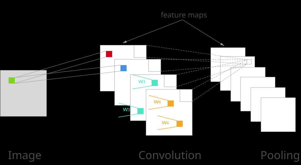
Figure 8.1: Convolution and Pooling Operations

Quiz: Pixel Context

Chapter 5’s k-NN classifier used only the RGB triple of each pixel and topped out near Dice ≈ 0.72 on the urothelial test set. Why is pixel-only classification fundamentally limited for cytology segmentation?

An RGB value alone cannot distinguish the edge of a cytoplasm from the interior of a faint nucleus — both can produce the same colour. Edges, textures, and nuclei are defined by patterns across neighbourhoods of pixels, information no single pixel carries

RGB has only three channels; switching to HSV would solve the problem because its three channels carry extra information that resolves the ambiguity

k-NN is too slow for image data — switching to a CNN is faster, and that speed-up is what improves segmentation quality

k-NN in RGB cannot handle grayscale images, and cytology images are stored as grayscale

8.2.2 Convolution by Hand

Let us compute a convolution directly — no library, just a nested loop — so the machinery is transparent.

import numpy as np

def manual_conv2d(image, kernel):
    """
    Apply a 3x3 kernel to a 2-D image.  Returns an output smaller by 1 pixel
    on each side (no padding).

    image  : (H, W) float array
    kernel : (3, 3) float array
    """
    H, W = image.shape
    output = np.zeros((H - 2, W - 2))   # output shrinks: we need a full 3x3 neighbourhood

    for row in range(H - 2):
        for col in range(W - 2):
            patch = image[row : row + 3, col : col + 3]   # 3x3 window
            output[row, col] = (patch * kernel).sum()     # dot product
    return output

Reading the loop. For every valid (row, col) position we extract the 3×3 patch of the image centred near that point, multiply it element-wise with the kernel, and sum the nine products into a single output value. The output is smaller by one pixel on each side because we need a complete 3×3 neighbourhood around every output position.

Now apply three very different kernels to a grayscale crop of a urothelial cell:

# Blur kernel: uniform average of the 3x3 neighbourhood
blur_kernel = np.ones((3, 3)) / 9.0

# Horizontal edge kernel: +1 on top, -1 on bottom -> responds to horizontal edges
edge_kernel = np.array([[ 1,  1,  1],
                        [ 0,  0,  0],
                        [-1, -1, -1]], dtype=float)

# Random kernel: no special structure
rng = np.random.default_rng(7)
rand_kernel = rng.standard_normal((3, 3))

# gray7 is a grayscale crop of a cell image from Chapter 5
out_blur = manual_conv2d(gray7, blur_kernel)
out_edge = manual_conv2d(gray7, edge_kernel)
out_rand = manual_conv2d(gray7, rand_kernel)

What the three outputs show:

• Blur — smooths local noise; the cell boundary is still visible but softer. Output looks like a slightly out-of-focus version of the input.
• Edge — bright where intensity drops downward, dark where it rises; the horizontal edges of the nucleus light up clearly. The same kernel structure you saw as Sobel X in Chapter 7.
• Random — noisy salt-and-pepper image with no obvious meaning. Random weights encode no useful pattern.

This is the central question CNNs answer: what if, instead of picking kernel weights by hand, we let the network learn the weights that best separate our classes? Everything else in this chapter is engineering around that single idea.

Quiz: Weight Sharing

A 256×256 grayscale image fed to a fully-connected layer mapping to a 100-unit hidden layer requires ~6.5 million weights. A single 3×3 convolution uses just nine. Why is this enormous reduction not a loss of expressive power for image data?

The same kernel is reused at every spatial location — “weight sharing.” A pattern detector for an edge or texture is the same regardless of where it appears in the image, so the network only needs to learn it once. Translating those nine weights across all positions provides the spatial coverage a fully-connected layer would have wasted millions of parameters duplicating

A convolution is mathematically equivalent to a fully-connected layer; the parameter count is just stored more efficiently in memory by reusing the same nine numbers many times

Image data only contains nine independent dimensions of variation, so nine weights are sufficient to capture every possible pattern

The fully-connected layer needs millions of weights only at training time; at inference it converges to nine effective weights, which the convolution mirrors

8.2.3 Interactive Convolution Widget

Before we build a learning CNN, use the widget below to convince yourself of two facts that the rest of the chapter relies on:

1. Different kernels produce fundamentally different feature maps. Load the Blur, Edge H, Edge V, and Sharpen presets. Each kernel extracts a different aspect of the same image.
2. The kernel + threshold that gives the lowest Dice loss is the one best matched to the target. Edit the ground-truth mask or change the kernel weights and watch the Dice score change. Training a CNN is nothing more than a systematic, automatic version of this trial-and-error.

How to use the widget:

• Input image (left) — click any cell to cycle its intensity in 0.1 steps from 0.0 (black) to 1.0 (white). The default scene mimics a cell: dark nucleus in the centre (0.05–0.30), brighter cytoplasm ring around it (0.70–0.80), bright background at the edges (0.95).
• Ground truth (centre-left) — click any cell to toggle foreground (red = target class) and background (dark).
• Kernel (centre-right) — click any weight to edit it. Use the preset buttons for standard kernels.
• Run Convolution — animates the 3×3 kernel sliding across the image, filling in the feature map one position at a time.
• Threshold slider — turns the feature map into a binary prediction. Pixels above the threshold become foreground.
• Dice score — displayed live. Dice = 1.0 means the thresholded feature map exactly matches the ground-truth mask.

Key insight. The widget lets you manually search for the kernel + threshold combination that maximises Dice. A CNN does exactly this search automatically — but across many stacked kernels, tuning thousands or millions of weights via gradient descent. The next sections build the smallest such network in PyTorch.

8.2.4 A Minimal CNN in PyTorch

We now implement the smallest useful CNN for our three-class segmentation task. The architecture has just three convolutional layers, no pooling, and ends in a per-pixel 1×1 convolution:

Input  (batch, 3, 256, 256)                 ← RGB cell images
   → Conv2d(3, 16, 3, padding=1) + ReLU     ← 16 feature maps
   → Conv2d(16, 32, 3, padding=1) + ReLU    ← 32 deeper feature maps
   → Conv2d(32, 3, 1)                        ← 1×1 conv = per-pixel classifier
Output (batch, 3, 256, 256)                 ← 3-class logits per pixel

What happens to a batch of cell images, step by step. Suppose we feed the network a batch of N RGB cell images — a 4-D tensor of shape (N, 3, 256, 256). The first layer, Conv2d(3, 16, 3, padding=1), holds 16 separate kernels, each a tiny 3×3×3 block of learned weights (one 3×3 slice per colour channel). Each kernel slides across the image one pixel at a time; at every position it multiplies its 27 weights by the matching 27 RGB values under the window, sums them, adds a bias, and writes the result into a single output pixel. Repeating this for all 16 kernels at every spatial location produces 16 feature maps of size 256×256 per image, so the tensor becomes (N, 16, 256, 256). The ReLU that follows then sets every negative entry in those 16 maps to zero, leaving only positive evidence of the patterns each kernel responded to.

A closer look at padding=1. “Padding by 1” means adding one extra row and one extra column on every side of the image before the kernel runs. The 256×256 input is therefore enlarged into a 258×258 working buffer — yes, 258, exactly as you’d expect from “1 pixel all the way around.” When the 3×3 kernel then slides across this padded buffer, its centre can reach every original pixel without falling off the edge, but the output still shrinks by 2 (because the kernel cannot centre on the very last row/column of any unpadded array). Net effect: 258 → 256 → output is the same 256×256 as the input. What goes into those padded pixels? The simplest, and PyTorch’s default, choice: zeros, in every channel. A zero pixel contributes nothing to the kernel’s weighted sum at the boundary, so the convolution sees a clean “no signal” past the image edge. (Other strategies exist — copy the nearest pixel (“replicate”), reflect the image across the edge (“reflect”), or wrap around — but zero-padding is what padding=1 gives you, and it is what we use throughout this chapter.)

The second layer, Conv2d(16, 32, 3, padding=1), repeats the same operation one level deeper. It holds 32 kernels of shape (16, 3, 3): each kernel now reads from all 16 incoming feature maps simultaneously, weighting and summing them into a single new 256×256 output map. The result is a (N, 32, 256, 256) tensor — 32 mid-level feature maps that combine and recompose the low-level patterns the first layer detected. A second ReLU again clamps negatives to zero.

The final layer, Conv2d(32, 3, kernel_size=1), is a 1×1 convolution: each of its 3 kernels has shape (32, 1, 1) — no spatial extent at all. At every pixel it takes the 32-number feature vector for that pixel and produces 3 weighted sums, one per class (background, cytoplasm, nucleus). The output tensor has shape (N, 3, 256, 256): three per-pixel score maps, one per class, the same height and width as the input. These raw, unnormalised scores are called logits.

A small clarification on what “logit” means here, since it is easy to confuse with a probability. A logit is just a raw real number — it can be positive or negative, large or small, and three logits at the same pixel are not required to sum to anything in particular. So an output triplet at a single pixel might look like (0.5, 1.2, -0.4). Higher means “more like this class,” but the three values are not yet probabilities. To get a probability triplet — three numbers in [0, 1] that do sum to 1, like (0.30, 0.60, 0.10), where the 0.60 reads naturally as “this pixel is about 60 % likely to be cytoplasm” — we apply the softmax function to the logits. Softmax is introduced in detail at the end of this section.

How the segmentation mask is computed. To turn the logits into the actual segmentation mask, we take the argmax along the channel dimension at every pixel: for each (row, col) location we look at the three logit values stacked there and pick the class index with the largest one. The result is an integer mask of shape (N, 256, 256) where every pixel carries a label 0 (background), 1 (cytoplasm), or 2 (nucleus). Drawn back onto the input as a colour overlay, that mask is the segmentation. (At training time we instead pass the raw logits straight into the cross-entropy loss, which internally applies a softmax to convert logits into class probabilities — the soft probabilities are needed to compute meaningful gradients. We only take the hard argmax at inference time, when we want a single class label per pixel.)

Softmax: turning logits into probabilities. The softmax function takes a vector of \(K\) real numbers (the logits) and returns a vector of \(K\) values in \([0, 1]\) that sum to 1 — a probability distribution over the \(K\) classes. For a logit vector \(\mathbf{z} = (z_0, z_1, \dots, z_{K-1})\), the \(k\)-th softmax output is

\[\text{softmax}(\mathbf{z})_k \;=\; \frac{e^{z_k}}{\displaystyle\sum_{j=0}^{K-1} e^{z_j}}.\]

Two things are happening in that formula. The exponential \(e^{z_k}\) makes every score positive — probabilities cannot be negative — and it amplifies differences: a logit one unit larger than another becomes about \(e \approx 2.7\) times bigger after exponentiation, so softmax pulls the distribution toward the largest logit. The denominator then divides by the total so the three (or in general \(K\)) outputs add to exactly 1. As a concrete instance, logits \((0.5,\, 1.2,\, -0.4)\) pass through softmax as

\[\frac{(e^{0.5},\, e^{1.2},\, e^{-0.4})}{e^{0.5} + e^{1.2} + e^{-0.4}} \;\approx\; \frac{(1.65,\, 3.32,\, 0.67)}{5.64} \;\approx\; (0.29,\, 0.59,\, 0.12),\]

an almost-(0.30, 0.60, 0.10) probability triplet — the network’s confident vote for “cytoplasm.”

There is a useful link to the Interactive Convolution Widget above. That widget produced one response map and asked you to pick a single threshold: pixels above the threshold became “foreground,” pixels below became “background.” That worked because there was only one number per pixel and only two possible labels, so a single cutoff was enough. Our segmentation network has three numbers per pixel and three possible labels, and the natural multi-class generalisation of “compare against a threshold” is “softmax to probabilities, then pick the largest.” (Argmax over softmax is equivalent to argmax over the raw logits — softmax is monotone — which is why we can skip softmax at inference time and apply argmax directly to the logits.)

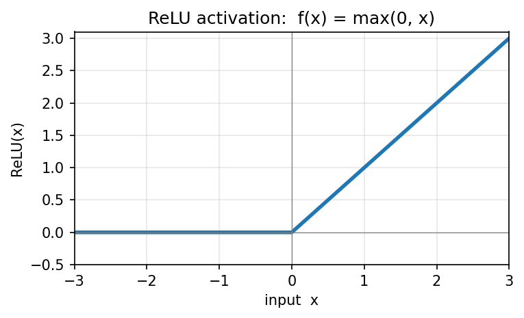
nn.ReLU (Rectified Linear Unit) is the activation function applied after the convolution. It is an element-wise operation:

\[\text{ReLU}(x) = \max(0, x)\]

Negative responses are clamped to zero; positive responses pass through unchanged. ReLU has no parameters of its own and does not change the shape of the tensor — only its values.

Figure 8.2: ReLU activation: f(x) = max(0, x)

ReLU’s job is to introduce non-linearity. Without it, two stacked Conv2d layers would mathematically collapse into a single (linear) convolution and the network could not learn anything richer than what one convolution already does. The chain Conv2d → ReLU is therefore the standard CNN building block — a learned linear filter followed by a simple non-linearity — and stacking many of them is what allows the network to compose progressively more abstract features (edges → textures → object parts).

import torch.nn as nn

class MinimalCNN(nn.Module):
    def __init__(self):
        super().__init__()   # required first line of any nn.Module subclass

        # Conv2d(in_channels, out_channels, kernel_size, padding)
        # padding=1 keeps spatial size the same when kernel_size=3
        self.conv1 = nn.Conv2d(3,  16, kernel_size=3, padding=1)
        self.conv2 = nn.Conv2d(16, 32, kernel_size=3, padding=1)
        self.conv3 = nn.Conv2d(32,  3, kernel_size=1)   # 1x1 conv

        self.relu = nn.ReLU()                            # max(0, x) activation

    def forward(self, x):
        # x: (batch, 3, 256, 256)
        x = self.relu(self.conv1(x))   # -> (batch, 16, 256, 256)
        x = self.relu(self.conv2(x))   # -> (batch, 32, 256, 256)
        x = self.conv3(x)              # -> (batch,  3, 256, 256), raw logits
        return x

What each layer does.

• conv1 learns 16 different 3×3 kernels applied jointly to the 3 RGB channels — 16 × (3 × 3 × 3 + 1) = 448 parameters. After training, these kernels often resemble edge detectors, colour-channel selectors, and simple texture detectors — essentially automatic versions of the Sobel and Gabor filters of Chapter 7.
• conv2 combines the 16 feature maps from conv1 into 32 deeper feature maps — 32 × (16 × 3 × 3 + 1) = 4 640 parameters. This layer learns mid-level features: corners, oriented patches, smooth regions.
• conv3 is a 1×1 convolution: at every pixel it takes the 32-channel feature vector and produces three class scores via a linear combination — 3 × (32 × 1 × 1 + 1) = 99 parameters. This is where the classification decision is made.

Total trainable parameters: 5 187. Compare with a fully-connected alternative: a single dense layer mapping a 256×256×3 image to even a modest 100-unit hidden layer would need 19.6 million weights. Convolution’s weight sharing is what makes the image-scale problem tractable.

Quiz: Why ReLU

The MinimalCNN inserts a ReLU activation between each pair of Conv2d layers. What goes wrong if you leave the ReLUs out and stack convolutions directly?

Two stacked linear convolutions are mathematically equivalent to a single (different) linear convolution — the composition of linear maps is still linear. Without a non-linearity between them, no matter how many layers you stack, the network can express only what one convolution can. ReLU is what lets the network compose progressively richer features (edges → textures → object parts)

Without ReLU the gradients become zero everywhere and training cannot progress at all — the network’s loss stays constant at its initialization value

Without ReLU the output values can become negative, and segmentation masks must be non-negative integers; ReLU is what enforces that constraint

ReLU acts like a dropout layer that randomly drops half of the activations during training; without it the network overfits immediately

8.2.5 Pooling

Pooling is the second standard CNN building block — distinct from convolution but often used alongside it. A pooling layer slides a small window (typically 2×2) across each feature map and replaces the values inside the window with a single summary number — usually the maximum (max-pool) or the average (avg-pool). The window stride is normally equal to its size, so windows do not overlap, and the spatial dimensions of the output therefore shrink: a 2×2 pool turns 256×256 into 128×128, a second one turns it into 64×64, and so on. Pooling is applied independently to each channel, so a (N, 32, 256, 256) tensor entering a 2×2 max-pool comes out as (N, 32, 128, 128): the channels are untouched, only the spatial grid shrinks.

Pooling and convolution differ on two crucial axes. Learnable parameters: a Conv2d layer stores trainable weights and biases and learns what patterns to detect; pooling has no parameters at all — it is a fixed summarising operation. Channel mixing: convolution combines information across channels (every output channel is a weighted sum over all input channels); pooling does not — every channel is summarised on its own. So convolution is the layer that learns features, while pooling is the layer that discards spatial detail to enlarge the receptive field cheaply.

Why use pooling at all? The receptive field — how much of the original input one output pixel depends on — grows much faster after pooling. After a single 2×2 pool, every subsequent 3×3 convolution effectively sees a 6×6 patch of the original image; after two pools, a 12×12 patch; after four, a 48×48 patch. This is how deeper networks aggregate evidence across whole nuclei or whole cells without exploding the kernel size. The cost is spatial precision: pooling collapses several pixels into one, and that fine-grained location information cannot be recovered. Our MinimalCNN deliberately omits pooling — every feature map stays at 256×256 — which keeps the architecture simple but caps the receptive field. Each output pixel depends on at most a 5×5 patch of the input (two stacked 3×3 convolutions), so a nucleus spanning 40 pixels cannot be perceived as a single object. Part 2 of this chapter introduces U-Net, which uses pooling to progressively grow the receptive field and then skip connections to recover the spatial precision pooling threw away.

NoteAll segmentation models are fully convolutional

Our MinimalCNN has no nn.Linear, no flatten, no global pooling — every layer is a 2-D convolution, and the output is a feature map the same spatial size as the input. This is the defining property of a Fully Convolutional Network (FCN): no fully-connected layers anywhere. Every modern segmentation architecture — U-Net, FPN, DeepLabV3+, PSPNet — is fully convolutional for exactly this reason: spatial structure must survive from input to output. A classification network (ResNet34, VGG, EfficientNet) is converted into a segmentation encoder by simply removing its final dense layers; what remains is an FCN.

Quiz: Pooling vs Convolution

Both pooling and convolution slide a window across feature maps, but they differ in two important ways. Which statement correctly describes the difference?

A convolution layer has learnable weights and combines information across all input channels into each output channel. A pooling layer has no learnable parameters and operates on each channel independently. Convolution learns what to detect; pooling discards spatial detail to enlarge the receptive field cheaply

Pooling is a special case of convolution with a 2×2 kernel of fixed weights \(\frac{1}{4}, \frac{1}{4}, \frac{1}{4}, \frac{1}{4}\). The two operations are mathematically the same, just named differently

Pooling has more learnable parameters than convolution because it must store the maximum from every window; convolution only stores nine weights per kernel

Pooling preserves spatial size while convolution shrinks it — that is why every CNN starts with pooling layers and ends with convolutions

8.2.6 Feeding the Network: Dataset Wrappers and DataLoaders

The MinimalCNN class above describes the model; before we can train it we still need a way to deliver data to it. PyTorch decouples these two concerns. A model accepts a tensor of shape (batch, 3, 256, 256) on its forward pass — but where do those batches come from? The answer is a small two-piece pipeline: a Dataset that knows how to fetch one sample, and a DataLoader that wraps it and yields batches.

The contract of a PyTorch Dataset is deliberately tiny — it requires only two methods:

• __len__(self) — the total number of samples available.
• __getitem__(self, i) — return sample number i as a (features, label) pair of tensors.

Anything that implements those two methods is a valid Dataset. PyTorch’s DataLoader will then call __len__ once to know the size of the dataset, and call __getitem__ repeatedly — possibly in parallel worker processes, possibly with a shuffled index order — collecting samples and stacking them into batches.

For our cell-segmentation problem the raw arrays X (shape (N, 3, 256, 256), float32 RGB images) and y (shape (N, 256, 256), integer masks with labels 0/1/2) already live in memory. We do not want to copy them into separate train/test arrays — that would double the memory footprint. Instead, we keep the full X and y once and pass each split as a list of indices into the original arrays. The wrapper looks like this:

# ── Dataset wrapper ───────────────────────────────────────────────────────────
# PyTorch requires a Dataset object that returns (image, label) pairs.
# __len__ returns the number of samples; __getitem__ returns one sample by index.
class SegDataset(Dataset):
    def __init__(self, X, y, indices):
        self.X = X
        self.y = y
        self.indices = indices

    def __len__(self):
        return len(self.indices)   # how many images in this split

    def __getitem__(self, i):
        idx = self.indices[i]
        # torch.from_numpy wraps a NumPy array without copying data
        img  = torch.from_numpy(self.X[idx])   # (3, 256, 256) float32
        mask = torch.from_numpy(self.y[idx].astype(np.int64))  # (256, 256) int64
        return img, mask

Walk through it line by line.

• class SegDataset(Dataset): — by inheriting from torch.utils.data.Dataset we get the abstract interface PyTorch’s DataLoader expects. Subclassing is required; the parent class itself does almost nothing other than mark the class as a Dataset.

• __init__(self, X, y, indices): — the wrapper does not own the image data; it merely keeps references to the full X and y arrays plus a list of indices belonging to this split (e.g. train_idx for the training set). Constructing a new SegDataset is therefore essentially free in memory — no copies are made.

• __len__(self): — returns len(self.indices), not len(self.X). This is what makes the wrapper a split: a training SegDataset reports only the number of training samples, even though it can see all of X.

• __getitem__(self, i): — this is the only place that actually reads data. The integer i ranges over 0 … len(self)-1; we look up the real index into X and y via idx = self.indices[i]. So when DataLoader shuffles, it shuffles the wrapper’s i, which we translate into a position in the original arrays.

• torch.from_numpy(self.X[idx]) — converts the NumPy slice into a torch.Tensor without copying. The tensor and the NumPy array share underlying memory: this is fast (no allocation) and means a tensor and the original array are kept consistent. The shape is (3, 256, 256) — already the channel-first layout PyTorch expects, so no transpose is needed.

• self.y[idx].astype(np.int64) — class labels must be int64 (a.k.a. torch.long) for nn.CrossEntropyLoss. The masks were stored as uint8 to save space, so we cast on the fly. The returned tensor has shape (256, 256) and contains integers 0, 1, or 2.

• return img, mask — every __getitem__ returns a (features, label) tuple. DataLoader expects exactly this two-tuple shape and stacks the firsts and the seconds separately into batched tensors of shape (batch, 3, 256, 256) and (batch, 256, 256) respectively.

With the wrapper in hand, building the actual loaders is a one-liner per split:

from torch.utils.data import DataLoader

train_loader = DataLoader(SegDataset(X, y, train_idx), batch_size=8, shuffle=True)
test_loader  = DataLoader(SegDataset(X, y, test_idx),  batch_size=8, shuffle=False)

shuffle=True on the training loader randomises the order of samples each epoch — important for stochastic gradient descent. shuffle=False on the test loader keeps the order deterministic so test metrics are reproducible. The batch_size=8 controls how many (image, mask) pairs DataLoader stacks before yielding a batch to the training loop. That training loop is what we look at next.

8.2.7 Training and Evaluation

The full training loop in PyTorch is short. The three lines that matter — forward pass, loss, backward pass — are the heart of every deep learning system:

import torch

device = torch.device('cuda' if torch.cuda.is_available() else 'cpu')
model  = MinimalCNN().to(device)

criterion = nn.CrossEntropyLoss()                            # standard multi-class loss
optimizer = torch.optim.Adam(model.parameters(), lr=1e-3)    # adaptive gradient descent

NUM_EPOCHS = 5
for epoch in range(NUM_EPOCHS):
    model.train()
    epoch_loss = 0.0
    for imgs, masks in train_loader:
        imgs, masks = imgs.to(device), masks.to(device)

        logits = model(imgs)                # forward pass
        loss   = criterion(logits, masks)   # compare to ground truth

        optimizer.zero_grad()
        loss.backward()                     # compute gradients via backpropagation
        optimizer.step()                    # update every weight slightly

        epoch_loss += loss.item()
    print(f'Epoch {epoch+1}  avg loss: {epoch_loss/len(train_loader):.4f}')

The three lines that matter.

1. logits = model(imgs) — forward pass. PyTorch runs all three convolution layers and returns per-pixel class scores, shape (batch, 3, 256, 256).
2. loss = criterion(logits, masks) — cross-entropy loss measures how far the predicted class distribution is from the ground-truth label at every pixel, then averages over the batch.
3. loss.backward() + optimizer.step() — PyTorch’s autograd engine computes \(\partial L / \partial w\) for every one of the 5 187 kernel weights, then nudges each weight in the direction that reduces loss. Thousands of these micro-updates later, the kernel weights have converged to values that separate the three classes well.

Test-set Dice comparison (per-image Dice averaged across the test split):

Method	Avg. Dice
Chapter 3 — hand-picked grayscale thresholds	≈ 0.48
Chapter 4 — Bayesian-optimised thresholds	≈ 0.58
Chapter 5 — k-NN in RGB space	≈ 0.72
Chapter 8 — MinimalCNN	≈ 0.84

Exact numbers vary slightly with the random seed; see VocEd Lab 05 for a full reproducible evaluation, including an N/C-ratio scatter that compares the four methods on the clinical quantity of interest.

Why the jump from 0.72 to 0.84? Two things changed at the same time:

1. The classifier now has access to spatial context — each pixel’s prediction depends on its 5×5 neighbourhood, not just its RGB value.
2. The kernel weights are learned for this specific task rather than picked by hand or fixed by a k-NN vote.

These factors compound. The 16 kernels in conv1 and the 32 kernels in conv2 specialise for patterns that help the final 1×1 classifier — exactly the patterns you were asked to search for manually in the widget above.

8.2.8 Tuning the MinimalCNN: Hyperparameters

The MinimalCNN reaches ≈ 0.84 Dice with the very first set of choices we tried — Adam at lr=1e-3, batch size 8, ReLU activations, 5 epochs, and hidden channel widths (16, 32) — i.e. Conv2d(3 → 16) → Conv2d(16 → 32) → Conv2d(32 → 3), where the leading 3 is the RGB input and the trailing 3 is fixed by the three-class task. Almost every one of those numbers was a guess. The settings that govern how the network is trained — but are not themselves learned — are called hyperparameters, and tweaking them can typically pull another 2–5 Dice points out of the same architecture, sometimes more. This subsection lays out which knobs are worth turning and how to decide which combination wins.

Learning rate — the size of each gradient-descent step. Too small and training crawls; too large and the loss diverges or oscillates. Useful values to try (with Adam):

• 1e-4, 3e-4, 1e-3 (current), 3e-3, 1e-2.

A practical rule for adaptive optimisers like Adam is to start near 3e-4; for plain SGD with momentum the sweet spot is usually 1e-2. Beyond a single fixed value, modern training almost always uses a schedule that lowers the learning rate over time:

• Step decay — multiply the rate by 0.1 every \(k\) epochs.
• Cosine annealing — smoothly decay from lr_max to near zero following a cosine curve.
• ReduceLROnPlateau — wait until the validation loss stalls, then drop the rate by a factor.
• One-cycle / warm-up — briefly raise the rate first, then decay; often gives the best final score for vision tasks.

The wrong learning rate is the single most common reason a deep network fails to train. If the loss is jumping around or stuck at its initial value, change this knob first.

Batch size — how many (image, mask) pairs are stacked into one gradient update. Useful values: 4, 8 (current), 16, 32, 64 — capped by GPU memory. Larger batches yield smoother, less noisy gradients and faster wall-clock training, but the noise of small batches is itself a mild regulariser that often improves generalisation. The interaction with learning rate is sharp: doubling the batch size, you typically need to (roughly) double the learning rate for SGD, or leave it alone for Adam. Tune the two together.

Optimiser type — the algorithm that turns gradients into weight updates. The Adam optimiser used above is the default for a reason, but there are several alternatives worth knowing:

• SGD with momentum (0.9) — the classic. With a good learning-rate schedule it often achieves the highest final accuracy on large vision datasets, at the cost of slower early progress. The combination “SGD + momentum + cosine annealing” is the recipe behind many ImageNet leader-boards.
• Adam / AdamW — adaptive per-parameter learning rates. Trains fast out of the box. AdamW is the modern variant in which weight decay is decoupled from the gradient update; it should be your default for any architecture using weight decay (which is virtually all transformers and most modern CNNs).
• RMSProp — the predecessor of Adam. Still common in recurrent networks and reinforcement learning.
• Lion (2023) — a newer optimiser from Google that uses only the sign of the momentum-smoothed gradient. Often matches AdamW with about half the memory and a slightly larger learning rate.
• Adafactor — memory-efficient adaptive optimiser used to train very large language and vision models.

For a small CNN like ours, Adam (or AdamW with weight_decay=1e-4) is almost always the right starting point.

Number of epochs — one epoch is one full pass over the training set. Five epochs is on the low end; the training loss is almost certainly still falling. Useful values: 10, 20, 50, 100. The right number depends on the gap between training loss and validation loss. Train until validation loss stops improving — this is the early stopping criterion — and then keep the best-performing checkpoint. Without early stopping, more epochs eventually start over-fitting: training loss keeps falling while validation loss climbs back up.

Activation function — the non-linearity inserted between layers. Alternatives to ReLU:

• Leaky ReLU — like ReLU but with a small negative slope (max(0.01·x, x)). Eliminates the “dying ReLU” problem in which a unit’s input stays negative forever and its weights stop updating.
• PReLU — same shape as Leaky ReLU but with the negative slope itself learned per channel.
• GELU (Gaussian Error Linear Unit) — smooth, used by every modern Transformer (BERT, GPT, ViT). About as cheap as ReLU.
• SiLU / Swish — x · σ(x), smooth, used by EfficientNet and many recent vision models. Often a small drop-in upgrade over ReLU.
• Mish — x · tanh(softplus(x)), smooth like Swish, sometimes a touch better at the cost of a bit more compute.
• ELU — exponential linear unit, smooth on the negative side, less popular today.

For a small CNN ReLU is hard to beat in practice; the smooth alternatives (GELU, SiLU, Mish) tend to help more in deeper networks.

Architecture — channel widths and depth. The hidden widths (16, 32) are arbitrary — the input has 3 channels (RGB) and the final layer must emit 3 channels (one logit per class), so only the interior widths are free to tune. Useful sweeps over those hidden widths:

• Narrower — (8, 16). About half the parameters; trains faster; risks under-fitting.
• Wider — (32, 64), (64, 128). More capacity; risks over-fitting and uses more memory and compute.
• Deeper — add a third hidden block: (16, 32, 64). Each extra Conv2d(3×3) adds two pixels to the receptive field.
• Larger kernels in the first layer — Conv2d(3, 16, kernel_size=5, padding=2) for a wider initial view of the image.
• Add Batch Normalisation (nn.BatchNorm2d) between conv and activation — usually allows a higher learning rate and more stable training at very little extra cost.
• Add Dropout (nn.Dropout2d(p=0.1)) — a regulariser that randomly zeros entire feature maps during training; helps when over-fitting.

Each of these is a hyperparameter — the number of hidden channels, the depth, the kernel size, the use of batch norm, the dropout rate. They all interact with everything above.

How to choose. Hyperparameters are picked by trying combinations and measuring validation performance — never test performance, which must remain untouched until the final report. The standard workflow:

1. Hold out a validation split from the training data (e.g. 80 / 10 / 10 train / val / test). Tune everything on val; report on test.
2. With small datasets, k-fold cross-validation gives a more reliable estimate. Split the training data into \(k\) folds (typically 5), train \(k\) models leaving one fold out at a time, and average the held-out scores. This costs \(k\) times more compute but reduces the noise in the validation signal.
3. Search strategies, in increasing order of efficiency:
   • Grid search — every combination on a discrete grid. Simple but the cost grows exponentially with the number of hyperparameters. Practical only for two or three at a time.
   • Random search — sample combinations randomly. Empirically beats grid search at the same compute budget — most hyperparameters do not matter much, and random sampling spends fewer experiments rediscovering this.
   • Bayesian optimisation — fit a surrogate model of the score as a function of the hyperparameters and use it to propose the next promising trial. This is the strategy you already used in Chapter 4 for picking the two thresholds, and it scales to a handful of continuous hyperparameters very well.
   • Hyperband / Successive Halving — start many configurations on a tiny budget (one epoch) and progressively reallocate compute to the survivors. Excellent when single trials are expensive.
4. Tune one knob at a time before reaching for a multi-dimensional search. The biggest gains usually come from learning rate and architecture width; epochs and activation function are typically lower-priority knobs.

A practical first sweep for the MinimalCNN: fix everything else, vary the learning rate over {1e-4, 3e-4, 1e-3, 3e-3}, and pick the one with the best validation Dice. Then sweep channel widths over {(8, 16), (16, 32), (32, 64)}. Two five-trial sweeps will already have you within a percentage point of the best configuration this architecture can deliver.

Diagnosing where the bottleneck lies — two channel-ranking strategies. Tuning the knobs above is more effective once you know which part of the network is holding back performance. After the MinimalCNN trains, every test image produces an activation tensor of shape (32, 256, 256) at conv2’s output: 32 channels, each a 256×256 map of per-pixel responses. Two simple rankings turn that mass of activations into a diagnostic. Strategy 1 — most active channels averages each channel’s activation magnitude across a held-out batch and sorts the 32 channels by the result; this tells you which channels the network uses heavily, regardless of what they detect. Strategy 2 — most class-relevant channels computes the point-biserial correlation between each channel’s flattened activation map and the flattened binary nucleus mask (y == 2), averaged across images. (Pearson correlation between a continuous variable and a binary 0 / 1 variable has a special name — point-biserial — but the formula is identical.) A high point-biserial coefficient means that the channel’s bright pixels coincide with nucleus pixels and its dim pixels coincide with non-nucleus pixels — the channel has learned to behave as a nucleus detector. Sorted top-down, this ranking surfaces the channels the network has internally allocated to the nucleus class.

Reading the two rankings together — upstream or downstream? The point of running both rankings is to localise where the model is failing. Suppose nucleus Dice is poor on the test set. Pair that observation with what Strategy 2 reports. If no channels show meaningful point-biserial correlation with the nucleus mask, the upstream pipeline (input → conv1 → conv2) never built a nucleus-aware representation in the first place — there is nothing for the final 1×1 classifier (conv3) to combine. The fix is upstream: widen the hidden channels, deepen the network, increase the kernel size, or change activations — interventions that expand the capacity of the feature extractor. Conversely, if Strategy 2 does surface several high-correlation channels but nucleus Dice is still poor, the upstream features are fine and the failure lies downstream in conv3 — the linear combination of channels into class logits — which calls for a different family of fixes: training longer, class-weighted cross-entropy, or sharpening the loss with a Dice term. Strategy 1 alone cannot make this distinction; a channel can be loud everywhere and still have zero point-biserial correlation. Combining the two rankings is what turns this section’s catalogue of hyperparameters from a shopping list into a guided search.

8.3 Part 2: U-Net for Cell Segmentation

NoteCompanion lab

Part 2 is paired with VocEd Lab 06 — U-Net: Multi-Scale Segmentation. The lab contains the runnable PyTorch code for the SmallUNet, the combined cross-entropy + soft Dice loss, the training loop, and the evaluation that produces the final entry in the cumulative Dice table. The code shown in this part is taken verbatim from that lab.

8.3.1 Why a Single-Scale CNN Isn’t Enough

The MinimalCNN of §8.4 reached ≈ 0.84 Dice on the test set despite being trivially small (5 187 parameters). It works because every pixel’s prediction can pool evidence from a 5×5 neighbourhood — already much better than the 1×1 vote of a k-NN classifier. But 5×5 is the upper limit: stack three 3×3 convolutions with padding=1 and you cap the receptive field at five pixels.

A urothelial nucleus, in our 256×256 images, typically spans 30–60 pixels — an order of magnitude larger than the receptive field. Two visible failure modes follow directly:

• Chromatin granules in cytoplasm look locally like nucleus. A small dark dot inside a cell body is identical, in a 5×5 window, to a fragment of a nucleus’s edge. The classifier has no way to see that the surrounding 50 pixels are uniformly cytoplasm.
• Large nuclei get fragmented. Pixels deep in the interior of a 50-pixel nucleus look locally like flat dark regions — interchangeable with shadow or empty background. Only by zooming out can the network confirm that those pixels belong to a connected nucleus.

The escape route is to pool the image down: stack convolutions and 2×2 max-pools so that one pixel of the deep representation summarises a much larger patch of the input. Pooling once gives a 10×10 effective view, twice gives 20×20, and so on.

But pooling alone destroys spatial precision. By the time the representation is at 64×64 with 128 channels, every “pixel” in the deep map covers a 4×4 region of the input — useful for classifying what is there, useless for drawing the boundary. The network needs the deep view (for context) and the shallow view (for precision) at the same time. That is what U-Net provides.

8.3.2 What “Receptive Field” Means

The phrase receptive field keeps appearing in this chapter, so it is worth pinning down precisely. The receptive field of a position in a feature map is the patch of pixels in the original input image whose values can possibly influence the value at that position. Anything outside the receptive field is invisible to that activation, no matter what the network has learned.

For segmentation, the receptive field is exactly the region of evidence each output pixel is allowed to use when it casts its per-class vote. If a nucleus is 50 pixels across but each output pixel sees only a 5×5 input patch, the network simply cannot use the nucleus’s full shape to decide what the pixel is — that information is outside its field of view.

Two simple rules govern how the receptive field grows as you stack layers:

• A k×k convolution with stride 1 adds k−1 to the receptive field. Two stacked 3×3 convolutions therefore see a 1 + 2 + 2 = 5-pixel patch — the second conv reads a 3×3 patch of the first conv’s output, and each of those 9 pixels was itself produced from a 3×3 input patch, so the union is 5×5.
• A stride 2 operation (max-pool 2×2, or a strided conv) doubles the step with which every subsequent conv extends the field. After one pool, every later 3×3 conv adds 2 × (3−1) = 4 input pixels instead of 2; after two pools, 4 × 2 = 8; after four, 16. Pools are the cheap way to grow the field — they have no parameters, yet a single one quadruples the per-conv reach.

Tracing the two networks of this chapter side-by-side makes the growth concrete:

Layer	MinimalCNN	SmallUNet (down to the bottleneck)
start	1	1
Conv 3×3 ×2 (enc1 block)	5 (after conv1 + conv2)	5
MaxPool 2×2	—	6 (step doubles to 2)
Conv 3×3 ×2 (enc2 block)	—	14 (at step 2)
MaxPool 2×2	—	16 (step doubles to 4)
Conv 3×3 ×2 (bottleneck block)	—	32 (at step 4)
Conv 1×1 (output head)	5 (unchanged — 1×1 adds 0)	—

So MinimalCNN tops out at 5×5 input pixels per output pixel — period. SmallUNet’s bottleneck sees 32×32 input pixels per bottleneck position; after the decoder’s two further ConvBlocks extend the field along the deep path, the output of SmallUNet reads from roughly 44×44 input pixels. That is the order-of-magnitude advantage U-Net buys you, and the reason kernel size (3×3) and receptive field (5×5 vs 44×44) are very different things.

8.3.3 Interactive Pooling Widget

Before we move on to the U-Net’s architecture, the widget below makes the mechanics of pooling concrete. Pooling is the operation in our forward method that does all the spatial-shrinking work — without it the encoder could not grow its receptive field at all — and it is genuinely simple once you watch it run.

How to use the widget:

• Input feature map (left) — an 8×8 grid of intensities. Click any cell to cycle its value through 0.0 → 1.0 in 0.1 steps. Use the preset buttons for ready-made scenes.
• Pool type — toggle between Max-pool (keep the largest value in each window) and Avg-pool (keep the mean of the four values).
• Run Pooling — animates a 2×2 window stepping across the input without overlap (stride 2), filling in the output one cell at a time. For max-pool, the winning input cell is briefly outlined in red so you can see which of the four pixels survived.
• Output feature map (right) — half the spatial size in each dimension. Eight rows become four; eight columns become four; sixteen 2×2 windows produce sixteen output values.

Three things to convince yourself of by playing with the widget:

• Pooling has no learnable parameters. Switching between max-pool and avg-pool changes the operation, not any weight. There is nothing inside a MaxPool2d(2) for gradient descent to update — it is a fixed summary, applied identically to every channel.
• Pooling is destructive. Once you have collapsed four input pixels into one output pixel, the precise location of the winning value is gone. Max-pool remembers the largest value; avg-pool remembers the typical value. Neither remembers which of the four it came from. This is exactly why the U-Net needs skip connections — to feed the pre-pool, full-resolution feature map back into the decoder so the boundary information lost during pooling can be recovered.
• Pooling is the cheapest way to grow the receptive field. A single 2×2 pool doubles the step at which subsequent convolutions reach into the input; two pools quadruple it. Without pools, the bottleneck’s 32×32 view (from the previous subsection) would have been only 9×9.

With the downsampling half of the U now mechanical, we turn to the upsampling half — and to the broader pairing of encoder and decoder that gives the architecture its name.

8.3.4 Encoder vs Decoder: Two Halves of the Same U

Pooling is only half the story. A pure-encoder network — one that just keeps shrinking the spatial dimensions and growing the channel dimensions — would ultimately output a single, deep feature vector summarising “what is in this image.” That is precisely what an image classifier does: ResNet, VGG, EfficientNet all collapse a 224×224×3 input into a 1×1×N vector that votes for one of N classes. Useful, but useless for segmentation, where we need to assign a class to every pixel — at the original resolution.

Segmentation therefore demands a second stage that runs the encoder backwards. Where the encoder progressively compressed spatial dimensions while expanding channel dimensions, the decoder progressively restores spatial dimensions while contracting channel dimensions. The encoder is the question “what is in this image, broadly?” and the decoder is the answer “and here is exactly where every part of it sits.” One pool in the encoder must be matched by one upsample in the decoder; one ConvBlock(in → 2·in) must be matched by a ConvBlock(2·in → in) (modulo the extra channels that arrive on the skip connection). They are step-for-step mirror images.

The complementarity is what makes the U work. By itself the encoder is too coarse to draw boundaries; by itself a decoder applied to the raw input would have no semantic context to draw boundaries of. The two together form a single network whose layers progressively zoom out (encoder) and then progressively zoom back in (decoder), trading detail for context on the way down and trading context for detail on the way up. The deepest layer — the bottleneck — is the pivot point where “context” peaks and “detail” bottoms out; the output layer is where they have been re-balanced into a per-pixel decision.

If the encoder uses pooling to lose spatial dimensions, the decoder needs an inverse: a way to grow those dimensions back. The upsampling widget below shows what that inverse looks like in practice.

8.3.5 Interactive Upsampling Widget

Upsampling takes a small feature map and produces a larger one — in our case, doubling the spatial dimensions. There is no new information being injected; the new pixels can only be computed from the existing ones, which means there is a choice of how to fill the gaps. Two parameter-free choices are common, and the widget below lets you flip between them.

• Nearest-neighbor — each output pixel just copies the value of its single nearest input pixel. Each input pixel becomes a 2×2 block of identical output pixels. Fast and exact on the values themselves, but produces visible blocky “staircase” artefacts at sharp edges.
• Bilinear — each output pixel is a weighted average of the (up to four) nearest input pixels, with weights chosen by linear interpolation: closer input pixels count more, farther ones count less. Smoother results, at the cost of inventing values that did not exist in the input. This is what our SmallUNet uses — the calls F.interpolate(b, scale_factor=2, mode='bilinear', align_corners=False) in the decoder.

How to use the widget:

• Input feature map (left) — a 4×4 grid of intensities. Click any cell to cycle 0.0 → 1.0 in 0.1 steps; use the preset buttons for ready-made scenes.
• Mode — toggle between Bilinear (the U-Net default) and Nearest.
• Run Upsampling — animates each output pixel filling in, with the contributing input pixels outlined in orange. For bilinear that is up to four input cells per output; for nearest, exactly one.
• Output feature map (right) — 8×8, double the spatial size of the input in each dimension. Same image area, finer sampling.

Two things to convince yourself of by playing with the widget:

• Nearest-neighbor preserves exact values; bilinear creates new ones. Switch to nearest with the Sharp edge preset and watch every output value match an input value exactly — but the edge stays brutally sharp. Switch back to bilinear and you see new values — 0.43, 0.27 — that were never in the input, smoothly bridging the transition. Bilinear’s smoothing is precisely what makes it the better choice when the next operation (a ConvBlock) wants spatially smooth inputs to work with.
• Upsampling alone can never recover what pooling threw away. Whichever mode you pick, you can only re-arrange the 16 input values into a 64-cell output. The high-resolution detail that existed before the encoder pooled it down is gone — the decoder is reconstructing it from a coarser starting point. This is the structural limit that motivates the U-Net’s third trick: skip connections, which copy the encoder’s high-resolution feature maps directly across the U so the decoder has access to the detail it would otherwise have to invent. We turn to those next.

8.3.6 U-Net vs MinimalCNN: What Changed and Why

Before reading the code, it helps to lay the U-Net’s design choices side-by-side with the MinimalCNN of Part 1. The MinimalCNN was a flat, single-scale, convolution-only network; the U-Net of Lab 06 changes both how the data flows and how the optimisation is set up.

Architecture changes.

Aspect	MinimalCNN (Lab 05)	SmallUNet (Lab 06)	Why it should help
Spatial structure	Flat — every layer at 256×256	U-shape: 256 → 128 → 64 → 128 → 256	Multi-scale view: deeper layers see large structures, shallow layers keep precise edges
Receptive field	≤ 5×5 pixels	32×32 at the bottleneck, ≈ 44×44 at the output (along the deep path)	Whole-nucleus context becomes available — see What “Receptive Field” Means above
Per-block depth	1 conv per layer	2 conv per ConvBlock	Two stacked 3×3 convs ≈ one 5×5 conv with fewer parameters and an extra non-linearity
Normalisation	None	BatchNorm2d after every conv	Stabilises the activation distribution; tolerates higher learning rates and small batches
Downsampling	None	MaxPool2d(2) between encoder levels	Doubles the receptive field per level; cheaper than strided conv
Upsampling	None	F.interpolate(..., mode='bilinear') between decoder levels	Smoothly enlarges feature maps without learning extra weights (a learnable alternative is ConvTranspose2d)
Cross-scale routing	None	Skip connections (torch.cat) at every level	Lets the decoder combine what (deep) with where (shallow) at the same resolution
Output head	Conv2d(32, 3, 1)	Conv2d(32, 3, 1) (unchanged)	Same per-pixel classifier; the work is done by everything upstream
Trainable parameters	~5 200	~415 000	~80× more capacity — a double-edged sword (see Part 4)

The hyperparameters change too — lr drops from 1e-3 to 3e-4, batch_size halves from 8 to 4, epochs double from 5 to 10, and the loss adds a soft Dice term alongside cross-entropy. We come back to why each value was picked when we read the training loop in §8.9; for now, just note that none of the optimiser-level choices (Adam, ReLU) changed.

The expected payoff from each change is qualitative, not quantitative — how much extra Dice they buy depends on the dataset. On a clean, large dataset the U-Net’s extra capacity and multi-scale view typically add 5–15 Dice points over a flat CNN. On a tiny dataset like ours, the same changes can also hurt if the extra capacity overfits before it learns multi-scale structure — exactly what we will observe at the end of this part. With that warning in place, we are now ready to read the code.

8.3.7 The U-Net Architecture

U-Net (Ronneberger, Fischer, & Brox, 2015) was designed for exactly this trade-off. Its shape — encoder contracting on the left, decoder expanding on the right, skip connections bridging the two — has become the standard for biomedical image segmentation.

We use the small two-level U-Net from VocEd Lab 06 as our worked example. It is small enough to read in one screen and large enough to show every U-Net idea in action. Before we look at the code, three new pieces of vocabulary need to be added to the convolutions-and-pooling toolkit you brought from Part 1: the block, the encoder, and the decoder. The bottleneck is just the joining piece between them.

A block is a small, reusable bundle of layers — in our case two Conv2d → BatchNorm2d → ReLU cycles — wrapped once and reused five times. Every time you see ConvBlock(in, out) later, read it as: take an in-channel feature map, apply two consecutive 3×3 convolutions (with batch norm and ReLU after each), and emit an out-channel map of the same spatial size. Nothing inside the block changes height or width — that work happens between blocks.

The encoder is a stack of blocks separated by MaxPool 2×2 downsamplings — the “compress and understand” half. Our SmallUNet’s encoder is two blocks: ConvBlock(3, 32) at full 256×256 resolution, a pool to 128×128, then ConvBlock(32, 64). Each pool sacrifices spatial precision for a wider field of view at the next block.

The decoder is the mirror image: blocks separated by upsampling steps. At each level it takes the small, deep feature map from below, doubles its spatial size with F.interpolate(..., bilinear), staples on the matching encoder block’s high-resolution feature map (the skip connection we detail in the next subsection), and runs another ConvBlock to mix the two streams. The output lands back at the input’s original resolution, ready for the final 1×1 classifier.

The bottleneck is the single block sitting at the deepest point between the two — smallest spatial size (here 64×64), widest channel count (here 128). Structurally it is just another ConvBlock; it gets a separate name because it occupies the join.

Drawn on a page these pieces form a literal U: encoder down the left, bottleneck at the bottom, decoder up the right. Hence the name.

With the vocabulary in place we can read the code, starting with the building block itself.

The reusable conv block. Each level of the encoder and decoder applies two Conv2d → BatchNorm2d → ReLU sequences in series. Three details of this small unit are worth stating explicitly:

• Two convolutions per block, not one. Two stacked 3×3 convolutions compute the same effective 5×5 receptive field as a single 5×5 convolution, but with 2 × (3·3) = 18 weights per channel pair instead of 25, and with one extra ReLU between them — a small, free-of-charge boost in expressive power. This VGG-style doubling is now standard in segmentation backbones.
• BatchNorm2d after every conv, before the ReLU. Batch norm rescales each feature map across the batch so that activations stay in a well-conditioned range. With it, the network tolerates the smaller batch size (4) we use here and the slightly higher learning rates that BN allows; without it, U-Nets at this depth often fail to train at all in the first few epochs.
• ReLU(inplace=True). The inplace flag tells PyTorch to overwrite the activation tensor instead of allocating a new one — a small memory win that lets us fit a larger batch on the same GPU.

import torch.nn as nn

class ConvBlock(nn.Module):
    def __init__(self, in_ch, out_ch):
        super().__init__()
        self.block = nn.Sequential(
            nn.Conv2d(in_ch,  out_ch, kernel_size=3, padding=1),
            nn.BatchNorm2d(out_ch),
            nn.ReLU(inplace=True),
            nn.Conv2d(out_ch, out_ch, kernel_size=3, padding=1),
            nn.BatchNorm2d(out_ch),
            nn.ReLU(inplace=True),
        )

    def forward(self, x):
        return self.block(x)

The full SmallUNet. Two ConvBlocks in the encoder, one at the bottleneck, two in the decoder, and a 1×1 output head:

import torch
import torch.nn.functional as F

class SmallUNet(nn.Module):
    def __init__(self, num_classes=3):
        super().__init__()

        # Encoder
        self.enc1 = ConvBlock(3,   32)        # operates at 256×256
        self.enc2 = ConvBlock(32,  64)        # operates at 128×128
        self.pool = nn.MaxPool2d(2)           # halves height and width

        # Bottleneck
        self.bottleneck = ConvBlock(64, 128)  # operates at 64×64

        # Decoder — input channels = upsampled + skip
        self.dec2 = ConvBlock(128 + 64,  64)  # 128 from bottleneck + 64 skip
        self.dec1 = ConvBlock(64  + 32,  32)  #  64 from dec2       + 32 skip

        # 1×1 output head
        self.out_conv = nn.Conv2d(32, num_classes, kernel_size=1)

    def forward(self, x):
        s1 = self.enc1(x)                                        # (N, 32, 256, 256)  ← skip 1
        s2 = self.enc2(self.pool(s1))                            # (N, 64, 128, 128)  ← skip 2
        b  = self.bottleneck(self.pool(s2))                      # (N,128,  64,  64)

        u2 = F.interpolate(b,  scale_factor=2, mode='bilinear', align_corners=False)
        u2 = self.dec2(torch.cat([u2, s2], dim=1))               # (N, 64, 128, 128)

        u1 = F.interpolate(u2, scale_factor=2, mode='bilinear', align_corners=False)
        u1 = self.dec1(torch.cat([u1, s1], dim=1))               # (N, 32, 256, 256)

        return self.out_conv(u1)                                 # (N,  3, 256, 256)

Trace the shapes. Reading the forward method top to bottom, each line tells you what spatial size and how many channels the activation has:

Input            (N,   3, 256, 256)              ← RGB image
  enc1           (N,  32, 256, 256)  ──┐         ← skip 1 saved
  pool + enc2    (N,  64, 128, 128)  ──┼──┐      ← skip 2 saved
  pool + bottleneck (N, 128,  64,  64)    │  │
  upsample ×2    (N, 128, 128, 128)       │  │
  cat(skip 2)    (N, 192, 128, 128)  ←────┘  │
  dec2           (N,  64, 128, 128)          │
  upsample ×2    (N,  64, 256, 256)          │
  cat(skip 1)    (N,  96, 256, 256)  ←───────┘
  dec1           (N,  32, 256, 256)
  1×1 out_conv   (N,   3, 256, 256)              ← per-pixel class logits

The same ConvBlock class is used five times — only the (in_channels, out_channels) numbers change.

Why those exact channel counts? The convention is to double channels each time you halve spatial resolution. As you compress space you can afford more feature dimensions; the total tensor size stays roughly constant. The deeper layers can then dedicate channels to higher-level concepts (cell-vs-background, cytoplasm-vs-nucleus, edge-direction) while shallower layers keep the channel budget small and the spatial detail sharp.

Two design choices worth noticing in the forward method.

• nn.MaxPool2d(2) for downsampling. A 2×2 max-pool with stride 2 halves the spatial size by keeping the largest activation in each window. The simplicity is the point: pooling forces the network to commit to a coarser view, freeing the convolutions to focus on what to do at each scale. A learnable alternative — nn.Conv2d(in, out, kernel_size=3, stride=2, padding=1) — replaces both the conv and the pool with one strided convolution and is used in some modern variants; it tends to help only on very large datasets, where the extra weights pay for themselves.
• F.interpolate(..., mode='bilinear', align_corners=False) for upsampling. Bilinear interpolation doubles the spatial size by averaging the four nearest neighbours of each new pixel. The learnable alternative is nn.ConvTranspose2d (“deconvolution”), which can introduce checkerboard artefacts unless tuned carefully; bilinear upsampling followed by a regular Conv2d (which our dec2 / dec1 already provide) sidesteps the artefact problem and is what most modern U-Net variants use.

Total parameters. Counting all the Conv2d and BatchNorm2d weights gives ≈ 415 000 trainable parameters — about 80× more than the 5 187 of MinimalCNN. The capacity has a single source: the channel widths grow rapidly as the spatial resolution falls, so the bottleneck ConvBlock(64 → 128) alone holds the largest weight count of any single block in the network.

8.3.8 Skip Connections, Intuitively

The line torch.cat([u2, s2], dim=1) is what distinguishes U-Net from a plain encoder-decoder. At every decoder level it gives the next ConvBlock two complementary signals at once: what this region is — coarse, semantic, blurry — from the bottleneck path, and exactly where its boundary sits — high-resolution, locally precise — from the skip path. After concatenation dec2 sees 64 + 128 = 192 channels and dec1 sees 32 + 64 = 96; each kernel learns to combine the deep channels (for what) with the shallow ones (for where).

8.3.9 Loss and Metrics for Segmentation

Segmentation produces a label for every pixel, so the loss must be aggregated over pixels too. Cross-entropy from §8.5 still works — average the per-pixel loss across the (height × width × batch) tensor — but it has a known weakness: it cares equally about every pixel, even though most pixels are background. A model that predicts “background everywhere” will already have a low cross-entropy loss on a typical cytology image where 70 % of pixels are background.

The standard fix is to add a soft Dice loss alongside cross-entropy. The Dice coefficient measures region overlap:

\[\text{Dice}(P, T) = \frac{2 \, |P \cap T|}{|P| + |T|}\]

For a single class \(c\), treat the predicted softmax probability \(P_c\) as a “soft” mask in \([0, 1]\) and the ground-truth as a 0/1 mask \(T_c\). Then \(\text{DiceLoss} = 1 - \text{Dice}\), averaged over classes. Soft Dice rewards good shapes: a prediction that gets every pixel right except for a thin border still scores near 1.0; a prediction that catches the right region but with the wrong class scores 0.

A single combined loss with equal weight gives both signals:

def dice_loss(logits, targets, num_classes=3, smooth=1.0):
    """Soft Dice loss averaged over all classes."""
    probs    = torch.softmax(logits, dim=1)
    one_hot  = F.one_hot(targets, num_classes).permute(0, 3, 1, 2).float()
    loss     = 0.0
    for c in range(num_classes):
        p, t = probs[:, c], one_hot[:, c]
        intersection = (p * t).sum()
        denom        = p.sum() + t.sum()
        loss += 1.0 - (2 * intersection + smooth) / (denom + smooth)
    return loss / num_classes

ce_loss = nn.CrossEntropyLoss()

def combined_loss(logits, targets):
    return ce_loss(logits, targets) + dice_loss(logits, targets)

A related metric: IoU. Intersection-over-Union is similar but stricter:

\[\text{IoU}(P, T) = \frac{|P \cap T|}{|P \cup T|}\]

For any prediction, \(\text{IoU} \le \text{Dice}\) — Dice double-counts the intersection in its numerator. Both are reported in segmentation papers; Dice is more common in medical imaging.

8.3.10 Training the U-Net

The training loop in Lab 06 is structurally identical to the one in Part 1 — three lines per batch (forward, loss, backward) inside an epoch loop — but the four hyperparameters that govern how it runs are all different.

train_loader = DataLoader(SegDataset(X, y, train_idx), batch_size=4, shuffle=True)
test_loader  = DataLoader(SegDataset(X, y, test_idx),  batch_size=4, shuffle=False)

optimizer = torch.optim.Adam(model.parameters(), lr=3e-4)

NUM_EPOCHS = 10
train_losses = []

for epoch in range(NUM_EPOCHS):
    model.train()
    epoch_loss = 0.0
    for imgs, masks in train_loader:
        imgs, masks = imgs.to(device), masks.to(device)

        logits = model(imgs)
        loss   = combined_loss(logits, masks)   # CE + soft Dice

        optimizer.zero_grad()
        loss.backward()
        optimizer.step()

        epoch_loss += loss.item()

    avg_loss = epoch_loss / len(train_loader)
    train_losses.append(avg_loss)
    print(f'Epoch {epoch+1:2d}/{NUM_EPOCHS}  —  avg loss: {avg_loss:.4f}')

# Save the trained weights for re-use in Lab 07 (N/C-ratio pipeline)
torch.save(model.state_dict(), 'unet_weights.pt')

Reading top to bottom:

• batch_size=4. Halved from the MinimalCNN’s 8 because the SmallUNet’s intermediate tensors are bigger — the (N, 128, 64, 64) bottleneck and especially the (N, 192, 128, 128) post-concatenation tensor in dec2 would push memory well past a free-tier Colab GPU at batch size 8. Smaller batches also add gradient noise, which on a small dataset acts as a mild regulariser.
• lr=3e-4. A third of the MinimalCNN’s 1e-3. With BatchNorm in every block, the activations are already well-scaled, so a smaller learning rate makes the loss curve smooth without sacrificing convergence speed.
• NUM_EPOCHS = 10. Doubled from 5. The U-Net has 80× more parameters and a more complex loss surface, so it simply needs more passes to settle. The loss curve typically still slopes downward at epoch 10 — there is room for more.
• combined_loss — cross-entropy plus soft Dice, defined in the previous subsection. The loss landscape is now shaped by two signals at once, and each batch’s gradient is a sum of contributions from both.
• torch.save(model.state_dict(), 'unet_weights.pt'). The trained weights are checkpointed at the end. This file is the artefact that Lab 07 (N/C-ratio pipeline) will re-load to run inference on new microscopy fields, without retraining.

The corresponding evaluation cell in Lab 06 (omitted here for length) iterates the test loader, takes argmax over the logit channel at every pixel, and computes the per-image Dice; averaging across the test set gives the final number reported next.

8.3.11 Why 0.77 — and How to Push It Higher

Trained with the loop above on the 200-image cytology training set, SmallUNet reaches an average test Dice of about 0.77. We can now extend the table from §8.5:

Method	Avg. Dice
Chapter 3 — hand-picked grayscale thresholds	≈ 0.48
Chapter 4 — Bayesian-optimised thresholds	≈ 0.58
Chapter 5 — k-NN in RGB space	≈ 0.72
Chapter 8 — MinimalCNN	≈ 0.84
Chapter 8 — SmallUNet	≈ 0.77

That number is lower than the MinimalCNN’s, which deserves a moment of honesty. The U-Net’s architectural advantages — multi-scale view, BatchNorm, skip connections, combined loss — are real, but they are not a free lunch. Two things are working against the U-Net here:

1. Capacity vs. data. SmallUNet has ~80× more parameters than MinimalCNN. With only ~140 training images and no data augmentation, that capacity is largely wasted: the network has enough degrees of freedom to memorise the training set before it learns multi-scale structure.
2. The dataset is friendly to small receptive fields. Most nuclei in the curated cytology images fall within a 5×5–10×10 patch — already at or just past MinimalCNN’s effective receptive field. The U-Net’s ≈ 44×44 view exists, but most images do not need it.

The good news is that every one of these issues has a known fix. None of them changes the architecture; they tune the training — exactly the kind of hyperparameter knobs we catalogued at the end of Part 1.

• Data augmentation (largest expected gain). Random horizontal/vertical flip, ±15° rotation, small elastic deformation, and brightness/contrast jitter turn 140 images into effectively thousands. PyTorch makes this a one-liner with torchvision.transforms.v2 or albumentations. Augmentation is the single most impactful change for any small-data segmentation problem, and it usually adds 5–10 Dice points to U-Net-class models.
• Longer training with early stopping. Hold out 10 % of the training set as a validation split; train for 50 epochs (or until validation Dice plateaus); keep the best checkpoint. Combined with augmentation, the loss curves typically keep improving well past epoch 30.
• Regularisation. Add weight_decay=1e-4 to Adam (or switch to AdamW), and a small nn.Dropout2d(p=0.1) inside each ConvBlock. Both are direct counter-measures to over-fitting on a small dataset.
• Smaller architecture. A one-level U-Net (32 → 64 → 32) has roughly a quarter of SmallUNet’s parameters but keeps the skip-connection idea. On this dataset it sometimes outperforms the two-level version.
• Class-weighted or focal loss. Replace cross-entropy with a class-weighted variant (or focal loss, \(\gamma = 2\)) to push the network harder on the rare nucleus pixels. Mostly improves nucleus Dice, leaving cytoplasm Dice unchanged.
• Train / validation / test discipline. The 0.77 number was measured on the test set the model was tuned against — a small but real source of optimism. A clean three-way split would make the comparison with MinimalCNN more honest.

The U-Net’s true strengths — large nuclei, crowded fields, ambiguous boundaries — are rare in this curated dataset, but they appear immediately when the same SmallUNet is run on whole microscopy fields in Lab 07. Part 4 of this chapter returns to the broader question implicitly raised by the 0.77: when does going deeper — to a ResNet34-encoded U-Net with millions of parameters — actually start to pay off?

Quiz: Skip Connections

Why does the U-Net decoder still need skip connections from the encoder, even though it can already access the bottleneck features?

Each downsampling step discards spatial detail. The bottleneck has rich semantic context but coarse 64×64 resolution; skip connections from earlier encoder levels carry the high-resolution detail the decoder needs to draw precise boundaries.

Skip connections add extra learnable parameters that increase the network’s capacity and lower the training loss.

Without skip connections, gradients cannot flow back through the encoder, so the encoder’s weights would never be updated.

Skip connections normalise the feature maps so that batch statistics match between training and inference.

8.4 Part 3: Looking Inside the Models

Up to now we have built two networks, watched their training-loss curves drop, and quoted Dice numbers off a held-out test set — and treated everything between input and output as a black box. This part opens the box. We pull the learned weights off the trained models, run a single test image through SmallUNet and save every intermediate activation, and re-train a deliberately broken U-Net to confirm what we said skip connections were buying us. Once we know what the models are and how they behave, the existing two questions remain — what do they still get wrong, and what would change in production? — and we close the part on those.

8.4.1 Learned Kernels: What MinimalCNN Discovered

After 5 epochs of training, MinimalCNN’s first convolutional layer holds 16 small RGB kernels of shape (3, 3, 3) — 16 × (3×3×3 + 1) = 448 learned numbers. These are the network’s analogue to Chapter 7’s Sobel and Gabor filters: the patterns conv1 decided were worth detecting in the input. A one-line cell pulls them straight off the trained model:

kernels = mincnn.conv1.weight.detach().cpu().numpy()   # (16, 3, 3, 3)

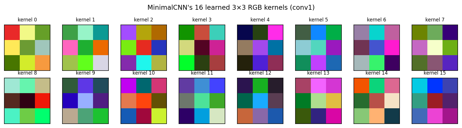
Plotting each kernel as a tiny RGB tile (per-kernel rescaled to \([0, 1]\) for display) gives:

Figure 8.3: MinimalCNN’s 16 learned 3×3 RGB kernels (conv1) after 5 epochs of training. Each tile shows one kernel; the three colour channels are packed back into RGB.

A few patterns are easy to read off:

• Colour-channel selectors — kernels that are nearly the same hue across all 9 cells. Their effect is to give the next layer access to a particular RGB combination (“more green than blue”, “red-minus-green”). These are how MinimalCNN reproduces what Chapter 5’s RGB k-NN was doing — but inside the network, automatically, instead of as raw input features.
• Spatial gradients — kernels with one bright row and one dark row, or one bright column and one dark column. These are Chapter 7’s Sobel edge detectors, reinvented from labelled data alone, and reinvented per-channel — something a hand-designed Sobel cannot easily do.
• Mixed colour-edge kernels — most of the rest. These respond jointly to colour and spatial structure, e.g. “red on the left, green on the right” — combinations that no single Chapter-7 filter expresses.

Nobody told MinimalCNN to detect edges or compare colour channels; it discovered both directly from 160 labelled cytology images. Compared with the Chapter 7 routine of choosing Sobel + Gabor + GLCM by hand, this is the chapter’s central claim made visible.

8.4.2 Feature Maps: An Image Through the U-Net

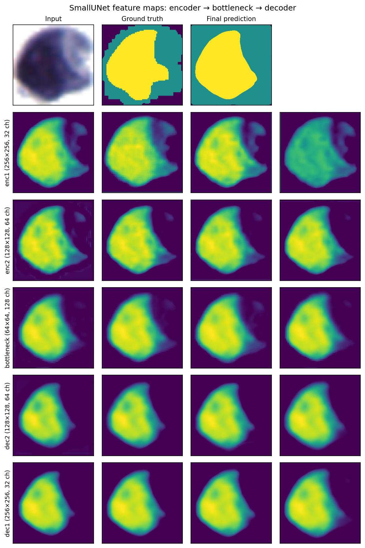
Kernels are what the network carries; activations are what the network does. Pick one cell from the test set, run it through SmallUNet, and capture every intermediate tensor. The figure below shows the input, the ground-truth mask, the network’s final prediction, and then the four most-active channels (by spatial variance) at each of the five internal stages.

Figure 8.4: Per-stage feature maps inside SmallUNet for a single test image. Top row: input, ground-truth mask, final per-pixel prediction. Below: four representative channels at each of enc1, enc2, bottleneck, dec2, dec1.

Reading top to bottom:

• enc1 (256 × 256, 32 channels). The first encoder block, still at full resolution. The cell is cleanly cut out from the background; edges are sharp; channels look like colour-biased copies of the input. This is what the kernels of conv1’s direct analogue actually do to the data.
• enc2 (128 × 128, 64 channels). After one max-pool. The spatial grid has halved, so each “pixel” here pools evidence from a 2 × 2 input window and the channels’ receptive fields stretch to ~14 input pixels. Local edges fade; overall cell shape dominates.
• bottleneck (64 × 64, 128 channels). The deepest stage. Spatial precision is gone — every activation summarises a 4 × 4 patch with a 32-pixel field of view — but the channels look like coarse, cleanly-divided maps of “nucleus”, “cytoplasm”, and “background”. This is the what signal the encoder was after.
• dec2 (128 × 128, 64 channels). The bottleneck has been bilinearly upsampled and concatenated with enc2’s skip. Spatial precision starts to come back; boundaries sharpen; channels are a hybrid of high-level semantic content and low-level edge information.
• dec1 (256 × 256, 32 channels). Full input resolution restored. Activations approximate a per-class soft probability map, ready for the 1 × 1 classifier on top.

The U-shape in the prose description shows up directly in the activations: spatial precision peaks at enc1, dies at the bottleneck, and is restored on the way back through dec2 and dec1. Without the skip connections, only the bottleneck’s coarse view would be available to draw the boundary from — which is the experiment we run next.

8.4.3 Skip Connections in Action

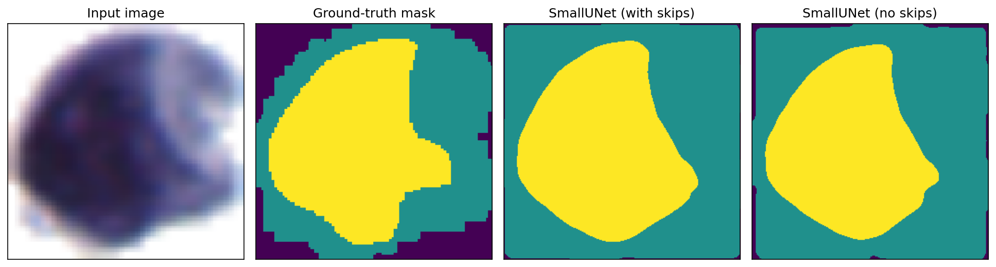
Up to now our argument for skip connections has been words: the bottleneck loses spatial precision, the skips feed it back. We can stop arguing and run the test directly. Define a no-skip variant of SmallUNet — same encoder, same bottleneck, same decoder layer count — but with the torch.cat([upsampled, encoder_features], dim=1) lines replaced by just the upsampled tensor. The decoder’s ConvBlocks shrink accordingly: dec2 becomes ConvBlock(128, 64) instead of ConvBlock(128 + 64, 64), dec1 becomes ConvBlock(64, 32) instead of ConvBlock(64 + 32, 32). Train it on the same 160 images for the same 10 epochs with the same combined loss, and run both networks on the same test image:

Figure 8.5: Same test image, two networks. The with-skip prediction follows the ground-truth boundary in detail; the no-skip prediction is a smoother, lower-resolution approximation.

Two things stand out:

1. Both networks find the cell. Coarse layout — where the cell sits in the field, where the nucleus lives inside it — is the same. The encoder–bottleneck pathway alone is enough for that.
2. Only the with-skip version draws the boundary at pixel-level precision. The no-skip prediction’s contour is a rounded approximation, like a low-resolution mask that has been stretched back up — exactly what it is, since the decoder had only the 64 × 64 bottleneck to work from. The with-skip prediction’s contour follows the ground-truth detail.

This is the what / where split made physical: both networks know what every region is; only the with-skip network knows where each boundary lies.

8.4.4 Evaluation and Failure Modes

Quantitative metrics (Dice, IoU, per-pixel accuracy) summarise overall performance, but they say little about what is going wrong. Qualitative inspection is essential.

Lab 06 ranks test images by per-image Dice and visualises the four worst predictions side-by-side with the ground truth and the original RGB image. Common failure patterns:

• Touching cells merge. When two nuclei touch at a single pixel, semantic segmentation cannot separate them — the network correctly predicts both regions as “nucleus” but cannot tell that they are two distinct objects. This is a fundamental limit of semantic (vs. instance) segmentation; the Instance Segmentation subsection in Part 4 discusses how to bridge the gap.
• Boundary imprecision near low contrast. Where the cytoplasm-to-background gradient is gentle, the predicted boundary jitters by a few pixels. This is unavoidable with a few-pixel ground-truth boundary annotation — the network is more precise than the labels.
• Small dark debris classified as nucleus. Chromatin fragments and stained dust both appear locally as “small dark regions.” Augmenting with explicit hard-negative examples (debris, slide artefacts) usually fixes this.

8.4.5 Deployment Considerations

Once the model is validated, two concerns drive its real-world use.

Domain shift. A network trained on slides from one microscope and one staining protocol will degrade on slides from a different lab. The fix is fine-tuning: take the trained weights, freeze most layers, and re-train the last few on a small batch of in-domain images. With as few as 20 new labelled images, performance typically recovers to within a few percentage points of the original.

Inference cost. SmallUNet runs in roughly 10 ms per 256 × 256 image on a modern GPU and ~200 ms on CPU. For batch processing this is irrelevant; for live microscopy it sets the cap on how many fields-of-view per second the system can analyse. Inference is bottlenecked by GPU memory more than compute — the skip-connection feature maps must all stay resident through the decoder pass.

8.5 Part 4: Where to Go Next

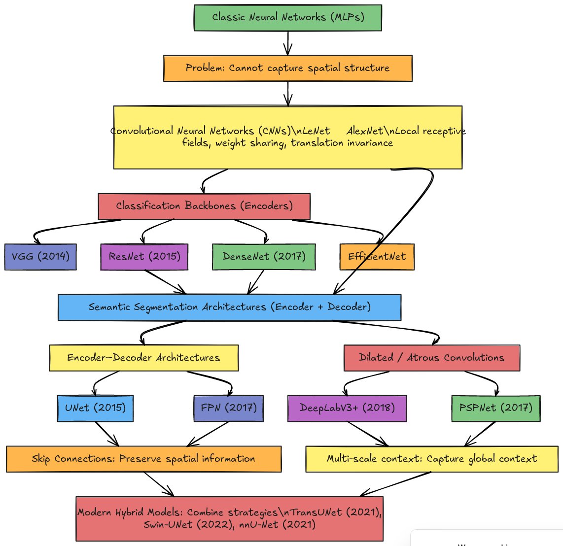
The MinimalCNN and U-Net are two specific points in a much larger architectural landscape. The flowchart below places them alongside the major families of image-analysis networks: classic MLPs; CNN-based classification backbones (VGG, ResNet, DenseNet, EfficientNet); encoder-decoder segmentation networks (U-Net, FPN); dilated-convolution architectures (DeepLabV3+, PSPNet); and modern hybrids that incorporate attention and transformer blocks (TransUNet, Swin-UNet, nnU-Net). This part takes the four directions you are most likely to encounter next — going deeper with residual networks, U-Net structural variants, multi-task heads, and instance segmentation.

Figure 8.6: Neural Network Architecture Evolution

8.5.1 Going Deeper: Residual Networks

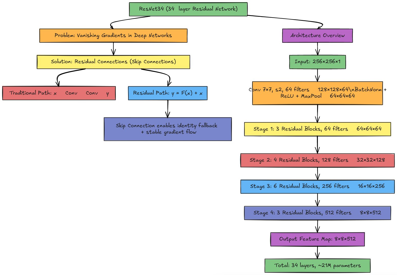
The benchmark above raises an obvious question: SmallUNet uses ~80× more parameters than MinimalCNN and gets a lower test Dice. Would going even deeper — say, with a 21-million-parameter ResNet34 encoder — help, or would it make the overfitting worse? On 200 images, almost certainly worse. Larger backbones help when the dataset is large enough to feed them (tens of thousands of training examples from scratch, or hundreds with strong ImageNet pre-training), when ImageNet pre-training transfers usefully (cytology stains are far from natural images — early layers transfer fine, late layers often don’t), and when the task rewards a much larger receptive field (wide-field histopathology, not 30–60-pixel nuclei in cleanly cropped cells). At the next scale of cytology screening — 5 000 annotated whole-slide images instead of 200 cropped fields — ResNet34 starts to dominate.

Residual blocks are what make depth tractable. Training very deep networks from scratch in 2014 ran into a paradox: 30-layer networks performed worse than 15-layer networks even on the training set. The culprit was the vanishing gradient problem — gradients are multiplied by each layer’s Jacobian on their way back through the network, so stacking thirty layers with multipliers slightly less than 1 leaves the gradient at the input layer at \(0.9^{30} \approx 0.04\) of its original size, too small to drive meaningful weight updates.

ResNet (He et al., 2015) fixed this with a remarkably simple change: instead of letting each block learn \(y = F(x)\), let it learn the residual \(F(x)\) from a baseline of “pass the input through unchanged”:

\[y = F(x) + x\]

Two consequences fall out. Identity is the default: if \(F\) collapses to zero, the block reduces to \(y = x\), so adding a block that has learned nothing leaves the signal alone. A gradient highway opens: the derivative of \(y = F(x) + x\) with respect to \(x\) is \(\frac{\partial F}{\partial x} + 1\), and the “+1” guarantees that gradients flow directly through the skip connection, bypassing the nonlinear path. Networks can now be 30, 50, or 100 layers deep without the early layers starving for gradient.

Input (x)
    │
    ├──────────────────────┐
    ↓                      │
3×3 Conv, BatchNorm, ReLU  │ (skip connection)
    ↓                      │
3×3 Conv, BatchNorm        │
    ↓                      │
    + ←────────────────────┘
    ↓
   ReLU
    ↓
Output (y = F(x) + x)

When channel counts change between stages (e.g. 64 → 128), a 1×1 convolution rescales the skip path so the channel counts match before the addition.

Plugging ResNet34 into U-Net. ResNet34 stacks 34 weighted layers as a stem and four stages of residual blocks — about 21 million parameters, hitting >70 % top-1 ImageNet accuracy when trained on its 1.2 million images.

Figure 8.7: ResNet34 Architecture

Stage	Blocks	Filters	Output (256² input)
Stem (7×7 conv stride 2 + 3×3 maxpool)	—	64	64 × 64 × 64
Stage 1	3	64	64 × 64 × 64
Stage 2	4	128	32 × 32 × 128
Stage 3	6	256	16 × 16 × 256
Stage 4	3	512	8 × 8 × 512

To use it in place of SmallUNet’s two-level encoder, tap the four ResNet stages as skip sources at resolutions 64, 32, 16, and 8 instead of 128 and 64; the decoder grows accordingly. With limited training data, load ImageNet-pretrained weights, freeze stages 1 and 2, and only fine-tune stages 3 and 4 plus the decoder. The PyTorch library segmentation_models_pytorch packages exactly this — smp.Unet(encoder_name='resnet34', encoder_weights='imagenet') is one line.

8.5.2 Variants of U-Net

U-Net has spawned a long list of variants tailored to specific challenges:

• Attention U-Net adds learned attention gates to each skip connection, so the decoder can choose which encoder features to attend to. Useful when the foreground is small or class-imbalanced.
• 3D U-Net extends the architecture to volumetric data (CT, MRI, confocal stacks) by replacing 2D convolutions and pooling with 3D operations.
• Recurrent U-Net adds RNN-style connections to model temporal coherence in video or time-lapse microscopy.
• Dense U-Net replaces residual connections with dense connections (DenseNet-style), concatenating all earlier feature maps within a block.

8.5.3 Multi-task Heads

The U-Net encoder learns features that are useful for many tasks beyond pixel-class prediction. Common multi-task setups for cytology:

• Segmentation + cell-type classification — share the encoder; one decoder head predicts the segmentation mask, a separate small classification head predicts a per-image cell-type label.
• Segmentation + boundary detection — a second 1×1 head predicts a soft edge map. Adding boundary supervision sharpens segmentation boundaries even when the main loss is on the mask.

8.5.4 Instance Segmentation

Semantic segmentation labels every pixel; it does not tell two touching nuclei apart. Three standard fixes for instance separation:

1. Connected components of the predicted nucleus mask. Cheap, but fails the moment two nuclei touch by even one pixel.
2. Watershed on a distance transform. Compute the distance to the nearest mask edge; treat it as a topographic map and let watershed flood from local maxima. Robust for slight contact.
3. Train a second head to predict boundary or distance maps. Use these as inputs to watershed. This is what Cellpose and StarDist do — instance-aware models that predict an auxiliary representation tailored to separating touching cells.

For a clinical N/C-ratio pipeline, instance segmentation matters whenever two cells touch within the field of view; the per-cell ratio is otherwise pooled across both, smearing the diagnostic signal.

8.6 Summary

This chapter built a segmentation pipeline from the ground up. We started with a single learned 3×3 kernel (the convolution widget), stacked three of them into the MinimalCNN, and saw test Dice jump from k-NN’s 0.72 to 0.84. The SmallUNet then added pooling for context and skip connections for spatial precision — but at 200 images it didn’t beat the simpler model. That tension is the point: the right architecture depends on the data you have, not on architectural fashion. Going deeper (ResNet34 + U-Net) is a real upgrade path, but only at a different scale of data.

The principles compound. Convolution + weight sharing makes images tractable; pooling builds context; skip connections preserve precision; residual blocks enable depth; and the choice of loss (cross-entropy + Dice) ties the gradient signal to the metric you actually care about. Every modern segmentation architecture — including the transformer-based ones we will not cover here — is built from these same pieces.